
Polynomial regression is very similar to linear regression, with a slight deviation in how we treat our feature-space. Confused? It'll make more sense in a minute, just bear with me.
As a reminder, linear regression models are composed of a linear combination of inputs and weights.
[{h _\theta }\left( x \right) = {\theta _0} + {\theta _1}{x _1} + {\theta _2}{x _2} + {\theta _3}{x _3} + ... + {\theta _n}{x _n}]
Polynomial regression is very similar, but it allows for a linear combination of an input variable raised to varying degrees.
[{h _\theta }\left( x \right) = {\theta _0} + {\theta _1}{x _1} + {\theta _2}x _1^2 + {\theta _3}x _1^3 + ... + {\theta _n}x _1^n]
Notice the difference? What if I told you that those were the exact same model? Don't believe me? Well, it's not always the case but suppose $x _2 = x _1^2$, $x _3 = x _1^3$, and so forth all the way to $x _n = x _1^n$. Clever right? So we can actually use linear regression models to perform polynomial regression by simply creating new features.
Polynomial regression is useful as it allows us to fit a model to nonlinear trends.
To do this in scikit-learn is quite simple.
First, let's create a fake dataset to work with. I've used sklearn's make_regression function and then squared the output to create a nonlinear dataset.
from sklearn.datasets import make_regression
X, y = make_regression(n_samples = 300, n_features=1, noise=8, bias=2)
y2 = y**2
Next, let's fit a linear model to the data and see how it performs.
from sklearn.linear_model import LinearRegression
model = LinearRegression()
model.fit(X, y2)
plt.plot(X, model.predict(X))
plt.scatter(X, y2)
plt.title("Linear Model, Polynomial Degree = 1")
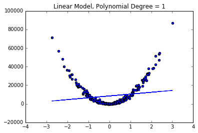
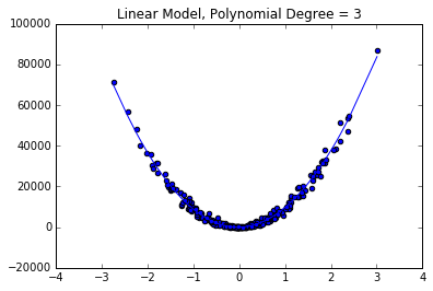
Not too impressive... However, if we create a couple polynomial features we can see a great improvement in our model's fit.
import numpy as np
from sklearn.preprocessing import PolynomialFeatures
poly_features = PolynomialFeatures(degree = 3)
X_poly = poly_features.fit_transform(X)
poly_model = LinearRegression()
poly_model.fit(X_poly, y2)

pred = poly_model.predict(X_poly)
new_X, new_y = zip(*sorted(zip(X, pred))) # sort values for plotting
plt.plot(new_X, new_y)
plt.scatter(X,y2)
plt.title("Polynomial Degree = 3")
A few practical notes on polynomial regression.
- Be careful of blindly using high-order polynomial models. These functions are generally not well-behaved and will produce dramatic unwanted fluctuations. Remember to use model evaluation techniques such as cross-validation to make sure your model generalizes well.
- Using a trick called regularization can prevent the aforementioned tendency for higher-order polynomial models to overfit the data in wild ways.