
Before you're ready to feed a dataset into your machine learning model of choice, it's important to do some preprocessing so the data behaves nicely for our model. In an ideal world, you'll have a perfectly clean dataset with no errors or missing values present. In the real world, however, such datasets are rare and uncommon. In this post, I'll be cleaning a dataset from Kaggle on Mental Health in Tech. I took a look at this dataset with my friend Florian (he's awesome, check him out here) earlier this year and decided it would serve as a good example for this post.
Inspecting the data
It's hard to know what to do if you don't know what you're working with, so let's load our dataset and take a peek. You can follow along in a Jupyter Notebook if you'd like.
import pandas as pd
import numpy as np

df = pd.read_csv("survey.csv")
num_columns = len(df.columns)
pd.set_option("display.max_columns", num_columns)
df.head(30)
The pandas head() function returns the first 5 rows of your dataframe by default, but I wanted to see a bit more to get a better idea of the dataset.
While we're at it, let's take a look at the shape of the dataframe too. Running df.shape will return information about the dimensionality of our dataframe (in this case it's the number of rows and columns), which will essentially tell you how many examples and features you are working with.
Pro tip: you can return the number of observations in your dataset with df.shape[0] and the number of features in your dataset with df.shape[1]. This is often helpful to do when building a model.
The first thing to understand is what features our dataset contains. You can read a description of each feature for this dataset on Kaggle.
Rather than inspecting each feature one-by-one, I opted for the lazier route and ran the following:
feature_names = df.columns.tolist()
feature_names.remove('Timestamp')
feature_names.remove('comments')

for column in feature_names:
    print column
    print df[column].value_counts(dropna=False)
This printed out a cell in my notebook with a ton of information about my dataset that I could easily consume by just scrolling through. As I looked through the dataset, I kept an eye out for things just as duplicate labels, erroneous or null values, and other things that just didn't quite seem right.
While many columns were fine as is, a couple columns needed cleaning. Here's a list of things I found that needed attention before feeding this model into a machine learning algorithm.
- The
Agecolumn contained people who had not been born yet (negative numbers). - The
Agecolumn also contained children (such as a 5 year old) that are unlikely to be taking a survey about their workplace. - The
Agecolumn contained someone who is 99999999999 years old, they should be in the Guiness World Records book or something. Jokes aside, this value is erroneous. - There are 49 different values listed for
Gender. Moreso, "Male" and "male" are ostensibly the same but currently being treated as two distinct categories. self_employedandwork_interferecontain some null values.
For numerical features, it can also be helpful to quickly examine any possible correlations between features. You can use the pandas scatter_matrix to easily visualize your data.
Separate the features and labels
If we're using a supervised machine learning technique, we need to make a distinction in the data between features and labels for each observation. Ultimately, this depends on what you're looking to predict or classify. In this case, I've decided that I'd like to build a classifier to predict whether or not someone will seek treatment.
features = df.drop('treatment', 1)
labels = df['treatment']
Cleaning null values (missing data)
Let's start with figuring out what to do with the null values found in self_employed and work_interfere. In both of these cases, the column contains categorical data. This is important to note the distinction between treating null values for categorical and numerical data, as the treatment will depend on the type of data present.
There's not exactly a formulaic way to approach how to treat missing data, as the treatment largely depends on the context and the nature of the data. For example, are the data missing at random or is there a hidden relationship between missing data and some other predictor?
One option in dealing with missing data is to simply ignore or remove the rows in which data is missing, discarding them from our analysis. However, this method is often unpopular due to the loss of information - especially if there was a pattern in your missing data.
A more method for handling missing values is imputation, where we replace the null value with our best guess of what that value might be. Basic implementations will simply replace all missing values with the mean/median/mode of all of the values for the given feature. More advanced implementations will use other features in order to develop an estimator for your missing value.
Take the following example, which is a small dataset containing three features (weather condition, temperature, and humidity) to predict whether or not I am likely to play tennis.
| Weather | Temperature | Humidity | Play tennis? | |
|---|---|---|---|---|
| 1 | cloudy | 60 | NaN | yes |
| 2 | rainy | 75 | 80% | NaN |
| 3 | cloudy | NaN | 50% | no |
| 4 | sunny | 65 | 40% | yes |
If we deleted all of the rows with null values we'd be left with one row, and our predictor would always guess that I would play tennis because that's the only example it has to learn from. Let's say we instead chose to replace the null temperature value in row 3 by mean imputation. In this case, row 3 temperature would be artificially reported to be 65. If we wanted to get fancier for replacing the null value for humidity in row 1, we could train an estimator to guess what the value might be given the weather and temperature data provided. It's important to note that with data imputation you are artifically reducing the variation in your dataset by creating new values close to (or equal to) the mean.
For a more in-depth analysis of techniques for treating missing data values, check out this chapter on missing-data imputation.
Scikit-learn provides an imputer implementation for dealing with missing data, as shown in the example below.
from sklearn.preprocessing import Imputer
imputer = Imputer(missing_values = 'NaN', strategy = 'mean', axis = 0)
imputer.fit(features)
features = imputer.transform(features)
Finding duplicate names
I mentioned earlier that there were 49 different values for 'Gender' and I suspected that some of these values should not be treated as distinct categories. Ultimately, I decided to resegment the data into 3 categories: male, female, and other (which accounts for non-binary and transgendered persons).
If I wanted to build a preprocessing engine which could clean incoming data, I could have probably taken a fancier approach and used some clever regular expressions to recategorize this column. Alas, I opted for the quick and dirty approach.
male_terms = ["male", "m", "mal", "msle", "malr", "mail", "make", "cis male", "man", "maile", "male (cis)", "cis man"]

female_terms = ["female", "f", "woman", "femake", "femaile", "femake", "cis female", "cis-female/femme", "female (cis)", "femail", "cis woman"]

def clean_gender(response):
    if response.lower().rstrip() in male_terms:
        return "Male"
    elif response.lower().rstrip() in female_terms:
        return "Female"
    else:
        return "Other"

df['Gender'] = df["Gender"].apply(lambda x: clean_gender(x))
Outlier detection
As I mentioned earlier, it seemed like there were some outlier values for Age which appear to be erroneous. Examples such as negative ages or extremely large integers could negatively affect the performance of our machine learning algorithm and we'll need to address them.
I went ahead and defined an acceptable range of ages for adults in the workplace and replaced numbers outside of this range with null values.
df.Age.loc[(df.Age < 18) | (df.Age > 80)] = np.nan
These null values could then be treated using the sklearn Imputer described earlier.
After defining a working range, I wanted to visualize the distribution of ages present in this dataset.
%matplotlib inline
import seaborn as sns
sns.set(color_codes=True)
plot = sns.distplot(df.Age.dropna())
plot.figure.set_size_inches(6,6)
Note: pandas has plotting capabilities built-in that you can use, but I'm a fan of seaborn and wanted to show that you have options when it comes to visualizing data.
Alright, at this point is seems like we're working with a pretty clean dataset. However, we're still not ready to pass our data into a machine learning model.
Encoding data
Many machine learning algorithms expect numerical input data, so we need to figure out a way to represent our categorical data in a numerical fashion.
One solution to this would be to arbitrarily assign a numerical value for each category and map the dataset from the original categories to each corresponding number. For example, let's look at the 'leave' column (How easy is it for you to take medical leave for a mental health condition?) in our dataset
df['leave'].value_counts(dropna=False)
which returns the following values.
Don't know            563
Somewhat easy         266
Very easy             206
Somewhat difficult    126
Very difficult         98
Name: leave, dtype: int64
In order to encode this data, we could map each value to a number.
df['leave'] = df['leave'].map({'Very difficult': 0, 'Somewhat difficult': 1, 'Don\'t know': 2, 'Somewhat easy': 3, 'Very easy': 4})
This process is known as label encoding, and sklearn conveniently will do this for you.
from sklearn import preprocessing
label_encoder = preprocessing.LabelEncoder()
label_encoder.fit(df['leave'])
label_encoder.transform(df['leave'])
The problem with this approach is that you're introducing an order that might not be present. In this case, one could argue that the data is ordinal ("very difficult" is less than "somewhat difficult" which is less than "somewhat easy" which is less than "very easy") but many times categorical data has no order. For example, if you had a feature for animal species, it doesn't make sense to assign values such than cats are less than dogs. The danger in label encoding is that your machine learning algorithm may learn to favor dogs over cats due to artficial ordinal values you introduced during encoding.
The common solution for encoding nominal data is one-hot encoding.
Rather than replacing the categorical value with a numerical value (label encoding) as shown below
| species | numerical encoding | |
|---|---|---|
| 1 | cat | 1 |
| 2 | dog | 2 |
| 3 | snake | 3 |
| 4 | cat | 1 |
| 5 | dog | 2 |
| 6 | turtle | 4 |
| 7 | dog | 2 |
we instead create a column for each value and use 1's and 0's to denote expression of each value. These new columns are often referred to as dummy variables.
| species | is_cat | is_dog | is_snake | is_turtle | |
|---|---|---|---|---|---|
| 1 | cat | 1 | 0 | 0 | 0 |
| 2 | dog | 0 | 1 | 0 | 0 |
| 3 | snake | 0 | 0 | 1 | 0 |
| 4 | cat | 1 | 0 | 0 | 0 |
| 5 | dog | 0 | 1 | 0 | 0 |
| 6 | turtle | 0 | 0 | 0 | 1 |
| 7 | dog | 0 | 1 | 0 | 0 |
You can one-hot encoding in directly in Pandas or use sklearn, although sklearn is a bit more convulted as the one-hot encoder only works for integer value inputs. For our example (where the inputs are strings), we would need to first perform label encoding and then one-hot encode the data.
# Using Pandas
import pandas as pd
pd.get_dummies(features['leave'])

# Using sklearn
from sklearn.preprocessing import LabelEncoder, OneHotEncoder
label_encoder = LabelEncoder()
ohe = OneHotEncoder(categorical_features = ['leave'])
label_encoded_data = label_encoder.fit_transform(features['leave'])
ohe.fit_transform(label_encoded_data.reshape(-1,1))
Feature scaling
At this point, we've successfully cleaned our data and converted it into a form which is easily consumable by machine learning algorithms. However, at this point we should consider whether or not some method of data normalization will be beneficial for our algorithm. This depends on (1) the data, (2) what we're trying to learn, and (3) the algorithm we plan to implement. Sometimes you'll need to revisit this step if you decide to change your machine learning algorithm.
The data
Suppose you have a dataset of features with different units: temperature in Kelvin, percent relative humidity, and day of year. If this dataset is representing weather values in Raleigh we might see the following ranges for each feature.
- Temperature: 270 K to 305 K
- Humidity: 0 to 1 (ie. 30% humidity represented by 0.3)
- Day of year: 0 to 365
When you're interpreting these values, you intuitively normalize values as you're thinking about them. For example, you recognize that an increase of 0.5 (remember: that's 50%) for humidity is much more drastic of a change than an increase of 0.5 Kelvin. However, if we don't scale these features our algorithm might learn to use temperature as the main predictor simply because it's scale is largest (and thus changes in temperature values are most significant to the algorithm). Feature scaling allows for all features to contribute equally (or more aptly, it allows for features to contribute relative to their importance rather than their scale).
What we're trying to learn
Sometimes, we'd like to be able to interpret our coefficients and changing the scale from something real (ie. dollars) to something arbitrary makes it more difficult to interpert our results.
The algorithm
If you're using a tool such as gradient descent to optimize your algorithm, feature scaling allows for a consistent updating of weights across all dimensions.
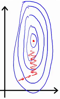
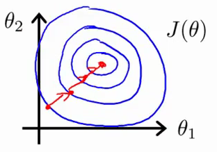
The following sketchs are borrowed from Andrew Ng's slides on gradient descent. The first image represents two features with different scales while the latter represents a normalized feature space. The gradient descent optimization may take a long time to search for a local optimum as it goes back and forth along the contours. A normalized feature space allows for much quicker convergence.
ML algorithms which require feature scaling:
- Logistic regression
- SVMs
- Perceptrons
- Neural networks
- PCA
ML algorithms which do not require feature scaling:
- Decision trees (and random forests)
- Naive Bayes
Note: the above lists are by no means exhaustive but simply serve as an example.
There's a few different methods for scaling features to a standardized range. Min-max scalers and standard scalers are two of the most commonly used approaches.
Min-max scaling sets your lowest observed value to 0 and your highest observed value to 1.
[{X_{sc}} = \frac{{X - {X_{\min }}}}{{{X_{\max }} - {X_{\min }}}}]
Standard scaling will convert the data to have a standard normal distrubtion.
[z = \frac{{X - \mu }}{\sigma }]
To do this (feature scaling) in practice, you can use pre-built libraries in sklearn.
# Feature scaling with StandardScaler
from sklearn.preprocessing import StandardScaler
scale_features_std = StandardScaler()
features_train = scale_features_std.fit_transform(features_train)
features_test = scale_features_std.transform(features_test)

# Feature scaling with MinMaxScaler
from sklearn.preprocessing import MinMaxScaler
scale_features_mm = MinMaxScaler()
features_train = scale_features_mm.fit_transform(features_train)
features_test = scale_features_mm.transform(features_test)
A few notes on this implementation:
- In practice, you may decide to only scale certain columns. For example, you don't need to scale the dummy variables from one-hot encoding.
- You'll want to scale your features the same for both the training and test sets (I'm getting ahead of myself here, stay tuned for the next section), so be sure to only transform the test set and not refit the scaler.
- I provided two ways to scale your feature set in the code above, choose one.
Splitting the data for training and testing
One of the last things we'll need to do in order to prepare out data for a machine learning algorithm is to split the data into training and testing subsets. Remember, machine learning is all about teaching computers to perform a task by showing it a lot of examples. We'll teach the computer using the data we have available, but ideally the algorithm will work just as well with new data. The principle behind the train/test split is to sacrifice some of the data for training in an attempt to evaluate the algorithm on "new" data it hasn't already seen. This is important because we want to ensure that our algorithm is able to generalize its learning from the given examples.
A nice analogy I heard once relates the concept to studying for a test. Let's say we have two students who are preparing for the same test- one student makes an effort to understand the general concepts that will be tested while the other student simply memorizes every example from the relevant homework sets. If the test contains new problems that weren't on the homework but are still related to the concepts discussed, the former student will perform much better on the test than the student who memorized the homework answers. In machine learning, we use the term overfitting to describe whether or not an algorithm has read too much into the data we provided as examples, or whether it was capable of generalizing the concepts we were trying to teach it.
Let's go ahead and split the data into two subsets (really it's four subsets, since we already separated features from labels).
from sklearn.model_selection import train_test_split
features_train, features_test, labels_train, labels_test = train_test_split(features, labels, test_size=0.25, random_state = 0)
Note: this will also shuffle your data. This is important if your data is ordered.
Validation data
When constructing a machine learning model, we often split the data into three subsets: train, validation, and test subsets. The training data is used to "teach" the model, the validation data is used to search for the best model architecture, and the test data is reserved as an unbiased evaluator of our model. When building a model, we often are presented with choices regarding the model's overall design; the validation data allows us to evaluate multiple designs in search of the best design, but in doing so we're "fitting" our model's design to this subset. Thus, the test data is still useful in determining how well our model will generalize what it learned to new data.
For machine learning problems with limited data, it's desirable to maximize the amount of data used to actually train your model. However, you must still hold out sufficient data for the validation set to evaluate model performance. In such situations, K-folds cross validation may come in handy.
For K-folds cross validation, we partition the dataset into $K$ bins. We will then run $K$ different learning experiments, each time choosing one bin as the evaluation subset while using the rest to train our algorithm. We can then average the results from all of the experiments to get an accurate picture of it's performance, using the entire dataset (albeit not at the same time) to both train and test the performance of our algorithm. Obviously, this approach will take more time, but it will give a more accurate evaluation of our machine learning model.
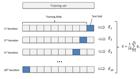
Image credit
Verifying consistent distributions across subsets
You'll get the best results if you're training and evaluating your data on data that has a similar distribution. Thus, it's best to verify this when splitting your data into subsets.
How much data is enough data?
Another useful thing to do at this stage is plot learning curves to judge whether or not you've collected sufficient data. These learning curves plot the training and validation scores of your algorithm for varying numbers of training examples.
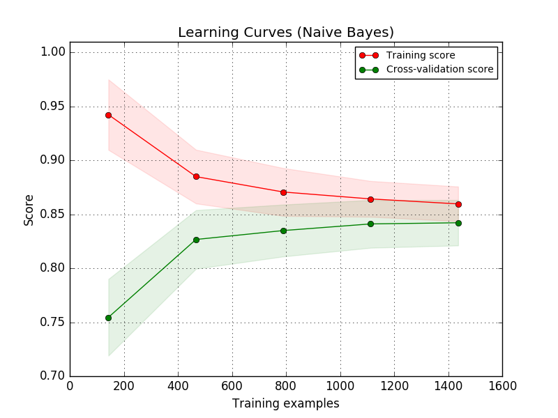
You will see that your model will plateau at a certain point and you'll begin to experience diminishing returns from adding additional training examples. This is primarily useful as it will tell you that you either need to go collect more data or that you've collected sufficient data and you shouldn't spend more time growing your dataset. For supervised learning, it can often be expensive to collect and label additional data for use in your model.
Note: this is where deep learning shines! Deep learning techniques are typically more capable of continuing to learn and improve the more data you feed it.
An example of sklearn's learning curve implementation can be found here.
The curse of dimensionality
Lastly, I'd like to briefly point out that simply throwing any and all information present at our machine learning algorithm generally isn't the best idea. This is commonly referred to as the curse of dimensionality, which observes that as the number of features in our dataset grow, the amount of data we need to accurately generalize grows exponentially.
Further reading
Combining features from different sources
How to Handle Missing Data
Kaggle course on feature engineering