
Principal components analysis (PCA) is the most popular dimensionality reduction technique to date. It allows us to take an $n$-dimensional feature-space and reduce it to a $k$-dimensional feature-space while maintaining as much information from the original dataset as possible in the reduced dataset. Specifically, PCA will create a new feature-space that aims to capture as much variance as possible in the original dataset; I'll elaborate on this later in this post.
Note: We're only dealing with the feature-space and not any corresponding labels or output. Dimensionality reduction is an unsupervised learning technique that is agnostic to the features' labels.
Let's start by addressing the burning question: how the heck do we reduce the dimensionality of our dataset? A naive approach might be to simply perform feature selection and keep only a subset of the original features. However, although we are reducing the dimensionality (we have less features), we're doing so by deleting information that might be valuable. A better approach would be to find a way to compress the information.
The ultimate goal with dimensionality reduction is to find the most compressed representation possible to accurately describe the data. If all of the features within your dataset were completely independent signals, this would be very hard. However, it's often the case that you will have redundancies present in your feature-space. You may find that many features are simply indicators of some latent signal that we haven't directly observed. As such, we would expect that indicators of the same latent signal would be correlated in some manner. For example, if we were trying to reduce the feature-space of a dataset that contained information about housing prices, features such as number of rooms, number of bedrooms, number of floors, and number of bathrooms all might be indicators of the size of the house. One might argue that these latent signals are the principal components which make up our dataset.
Intuition
Let's look at the following two-dimensional feature-space.
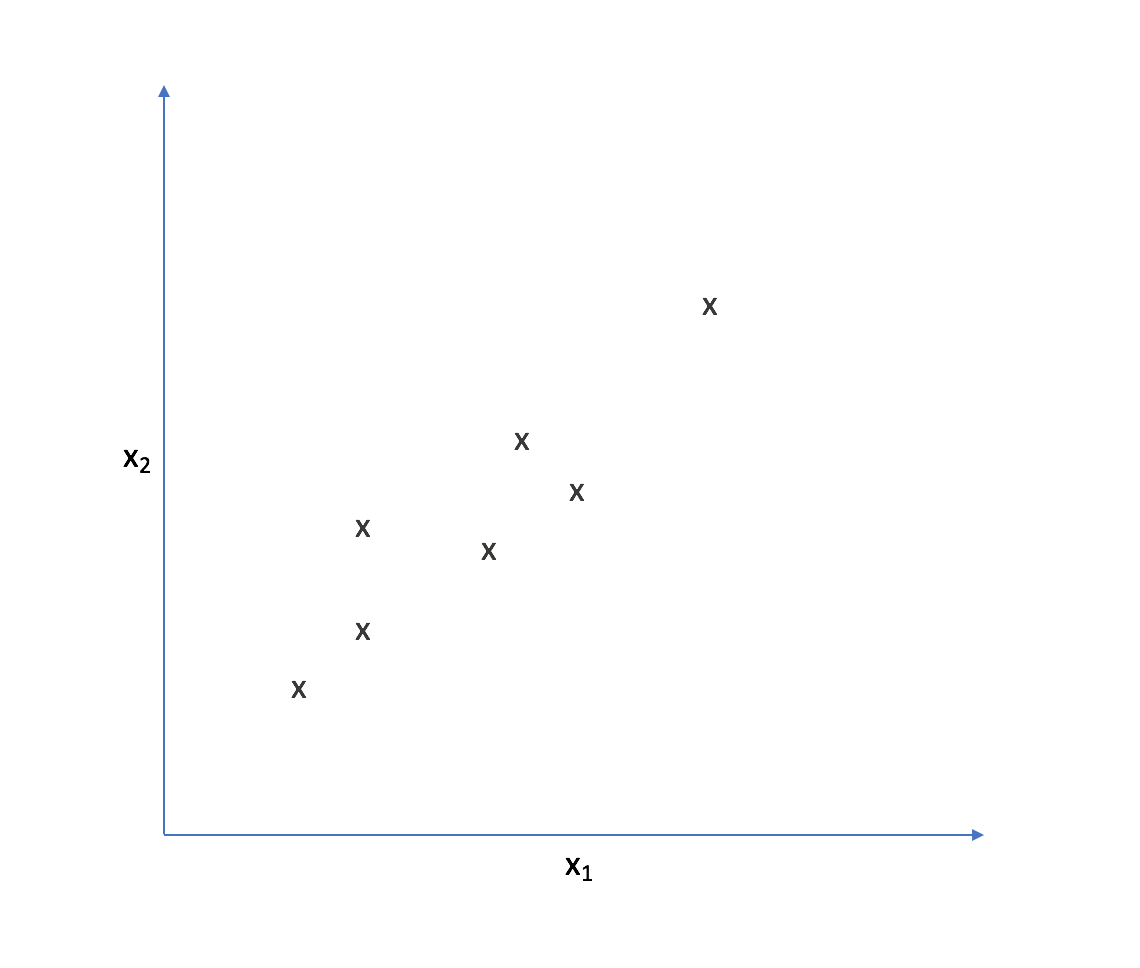
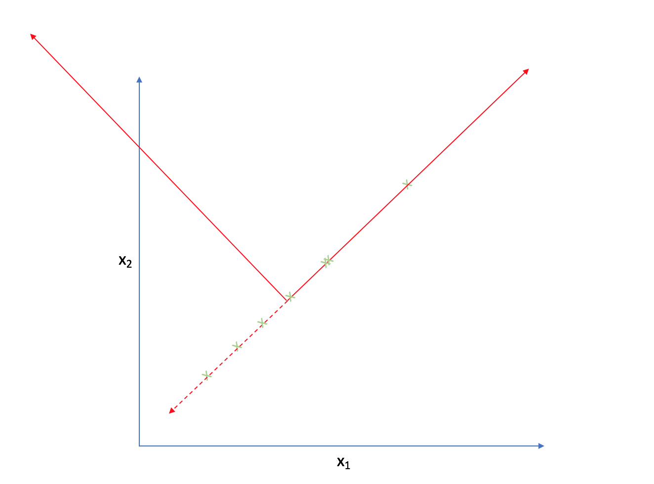
It appears that most of the points on this scatterplot lie along the following line. This suggests some degree of correlation between $x _1$ and $x _2$.
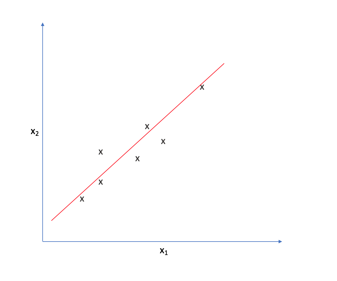
As such, we could reorient the axes to be centered on the data and parallel to the line above.
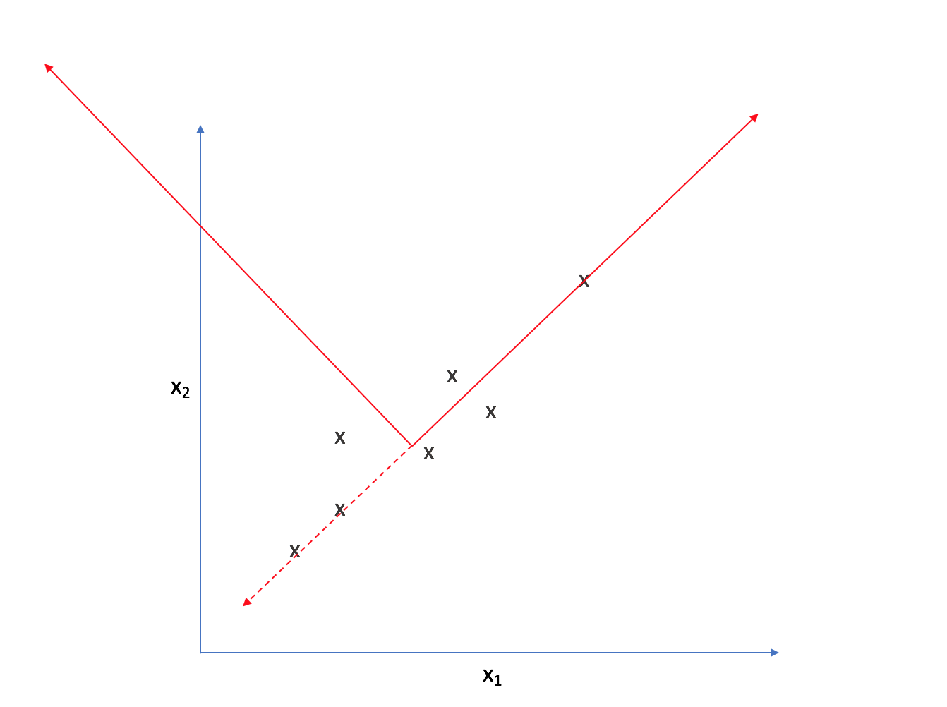
Strictly speaking, we're still dealing with two dimensions. However, let's project each observation onto the primary axis.
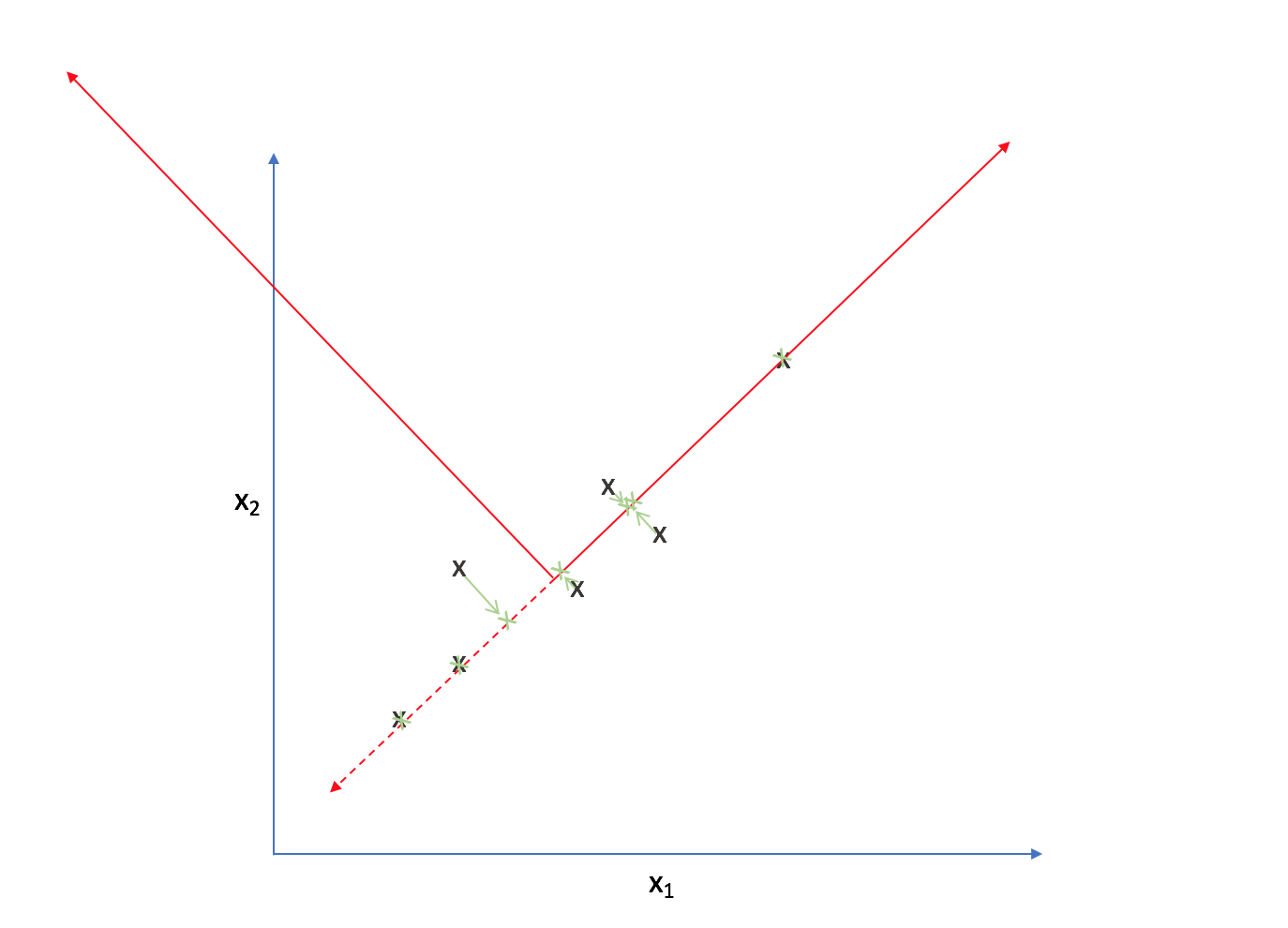
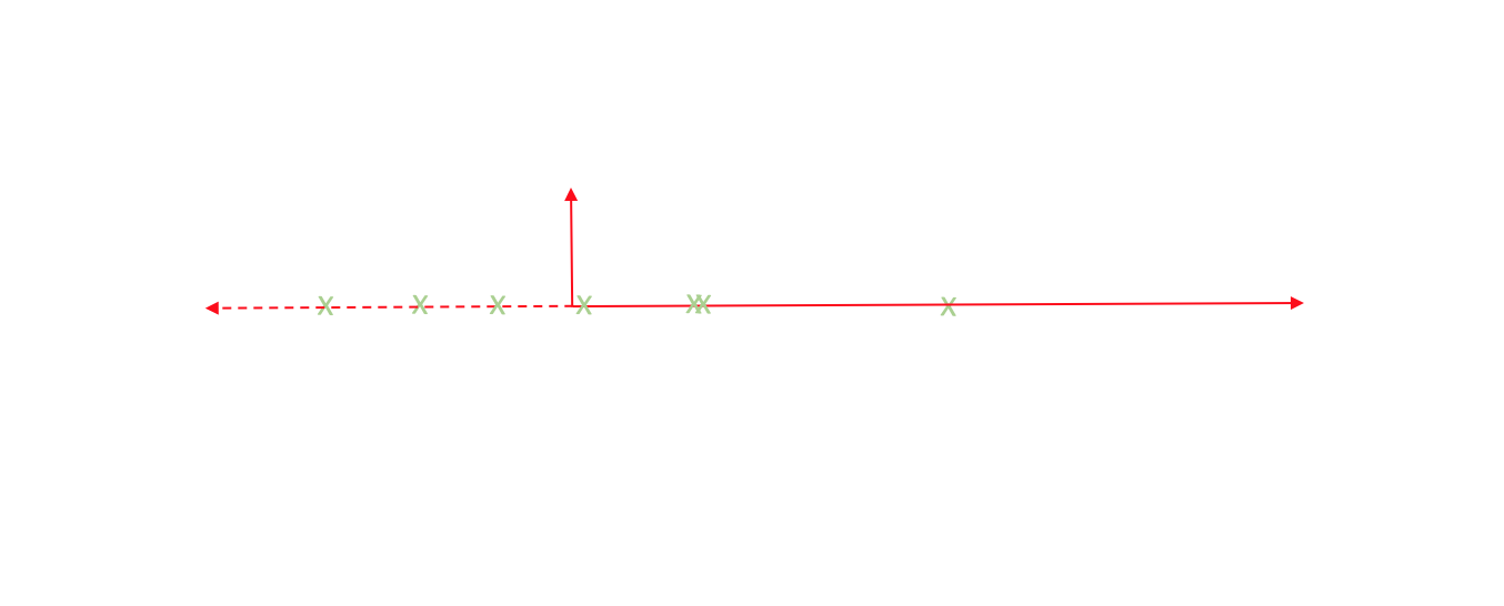
Now, every observation lies on the primary axis.
We just compressed a two dimensional dataset into one dimension by translating and rotating our axes! After this transformation, we only really have one relevant dimension and thus we can discard the second axis.
Boom. Dimensions reduced.
Comparing the original observations with our new projections, we can see that it's not an exact representation of our data. However, one could argue it does capture the essence of our data - not exact, but enough to be meaningful.
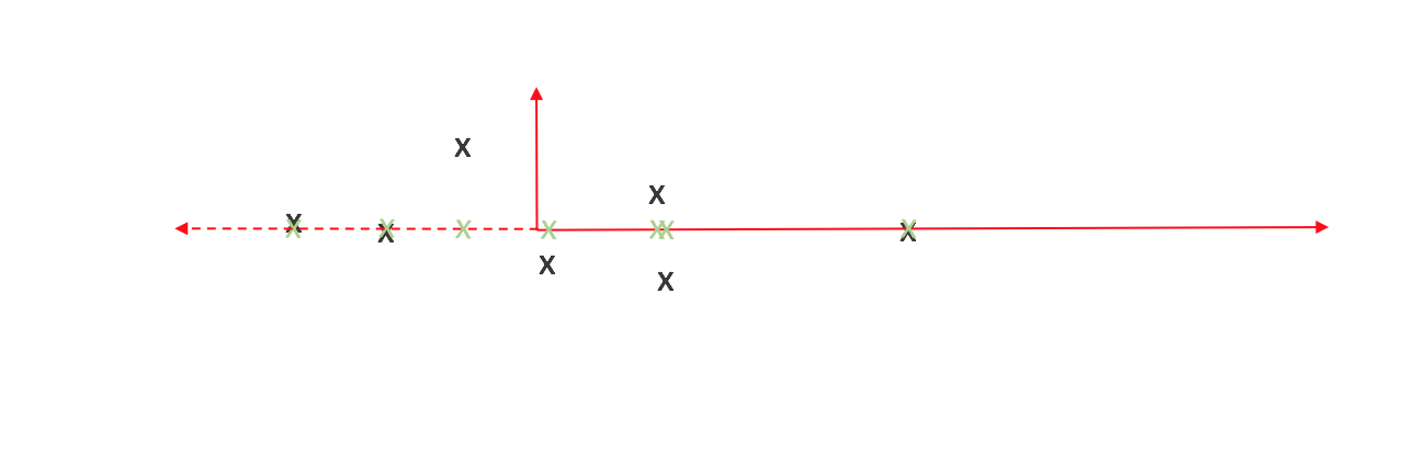
We can view the cumulative distance between our observations and projected points as a measure of information loss. Thus we'd like to orient the axes in a manner which minimizes this. How do we do this? That's where variance comes into play.
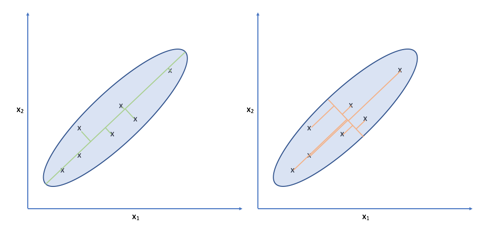
Let's take another look at the data. Specifically, look at the spread of the data along the green and orange directions. Notice that there's a much more deviation along the green direction than there is along the orange direction.
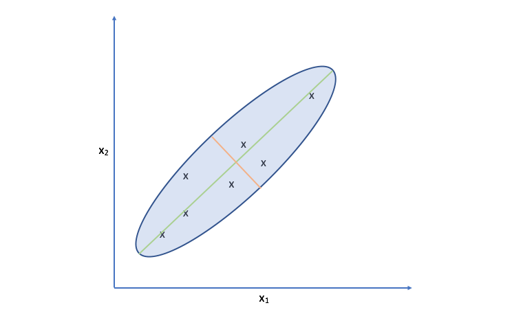
Projecting our observations onto the orange vector requires us to move much further than we would need to for projecting onto the green vector. It turns out, the vector which is capable of capturing the maximum variance of the data minimizes the distance required to move our observations as projection onto the vector.
Note: While this might look like linear regression, it is distinctly different. For one, linear regression measures error as the difference between the true output and the predicted output for a given input. This error is parallel to the y-axis. For PCA, there is no y-axis; we're doing unsupervised learning. Further, we measure error as the distance between the original observation and the projected observation along the direction of projection (orthogonal to the new axis).
More generally, we'd like to find a set of $k$ vectors on which we can project our data to reduce the feature-space from $n$-dimensions to $k$-dimensions. Further, we'd like to find these $k$ vectors such that we minimize the projection error or information loss; we earlier established that we can accomplish this by finding the direction of maximum variance within the data.
Algorithm
So far, we've established a method for reducing the dimensionality by finding the set of orthogonal vectors (through translation and rotation) which captures the maximum amount of variance within the data. Now, we'll discuss a way to achieve this algorithmically. This algorithm must contain a way to 1) find a new set of vectors to describe the data and 2) develop a way to project our original observations onto these vectors.
Before we transform our feature-space into such a representation, it's important that we normalize and scale the features. This allows variance to be a homogenous measure across all features.
The steps to perform PCA are as follows.
1. Compute the covariance matrix.
2. Find eigenvectors ($U$) and eigenvalues ($S$) of the covariance matrix using singular value decomposition.
[ {\left[ {U,S,V} \right]} = svd(\Sigma )]
3. Select $k$ first columns from eigenvector matrix.
4. Compute projections of original observation onto new vector form.
[z = U _{reduce}^Tx]
It's also possible to decompress $z$ and restore an approximation of the original feature-space.
[{x _{approx}} = {U _{reduce}}z]
We can compare this approximation to the original value in order to calculate the variance retained in our compressed feature-space. A common metric to evaluate our PCA feature compression is explained variance, which is another way of saying the amount of original variance by which our compressed representation is still able to retain. (Recall that we lost some variance of the data when projecting the observations onto the new vector in the 2D example.)
For example, if we were to compress our feature-space in a manner that retains 95% variance of the data, we could write:
[1 - \frac{{\frac{1}{m}\sum\limits _{i = 1}^m {{{\left| {{x _i} - {x _{i,approx}}} \right|}^2}} }}{{\frac{1}{m}\sum\limits _{i = 1}^m {{{\left| {{x _i}} \right|}^2}} }} \ge 0.95]
Choosing k
One method for choosing $k$ would be to start at $k=1$, and continue increasing $k$ until we drop below some set threshold of explained variance. This would involve calculating the explained variance for each iteration and is computationally inefficient.
A better approach to calculating $k$ is to leverage the eigenvalues ($S$) we found in singular value decomposition. While the eigenvectors represent the directions of maximum variance, the eigenvalues represent the magnitudes of variance in each corresponding direction.
This is quite convenient and it is much easier to use these magnitudes in calculating the explained variance for a given $k$.
[1 - \frac{{\frac{1}{m}\sum\limits _{i = 1}^m {{{\left| {{x _i} - {x _{i,approx}}} \right|}^2}} }}{{\frac{1}{m}\sum\limits _{i = 1}^m {{{\left| {{x _i}} \right|}^2}} }} = \frac{{\sum\limits _{i = 1}^k {{s _{ii}}} }}{{\sum\limits _{i = 1}^n {{s _{ii}}} }}]
Further reading
- Principal component analysis with linear algebra
- Interpretation of the Principal Components
- Linear algebra - Alternate coordinate systems
- Linear algebra - Eigenvectors
- Covariance matrix
- Singular Value Decomposition
- More slides on PCA
- Making sense of principal component analysis, eigenvectors & eigenvalues