
This post aims to discuss what a neural network is and how we represent it in a machine learning model. Subsequent posts will cover more advanced topics such as training and optimizing a model, but I've found it's helpful to first have a solid understanding of what it is we're actually building and a comfort with respect to the matrix representation we'll use.
Prerequisites:
- Read my post on logistic regression.
- Be comfortable multiplying matrices together.
Inspiration
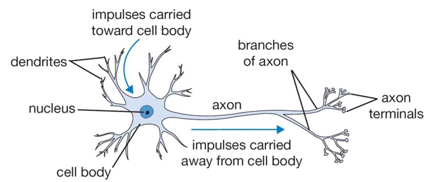
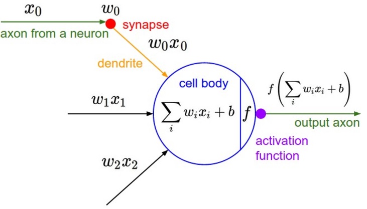
Neural networks are a biologically-inspired algorithm that attempt to mimic the functions of neurons in the brain. Each neuron acts as a computational unit, accepting input from the dendrites and outputting signal through the axon terminals. Actions are triggered when a specific combination of neurons are activated.
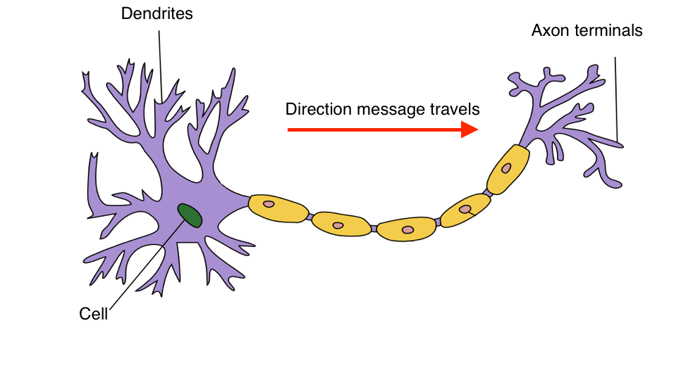
In essence, the cell acts a function in which we provide input (via the dendrites) and the cell churns out an output (via the axon terminals). The whole idea behind neural networks is finding a way to 1) represent this function and 2) connect neurons together in a useful way.
I found the following two graphics in a lecture on neural networks by Andrea Palazzi that quite nicely compared biological neurons with our computational model of neurons.
To learn more about how neurons are connected and operate together in the brain, check out this video.
A computational model of a neuron
Have you read my post on logistic regression yet? If not, go do that now; I'll wait.
In logistic regression, we composed a linear model ${z\left( x \right)}$ with the logistic function ${g\left( z \right)}$ to form our predictor. This linear model was a combination of feature inputs $x_i$ and weights $w_i$.
$$ z\left( x \right) = {w_1}{x_1} + {w_2}{x_2} + {w_3}{x_3} + {w_4}{x_4} + b = {w^{\rm{T}}}x + b $$
Let's try to visualize that.
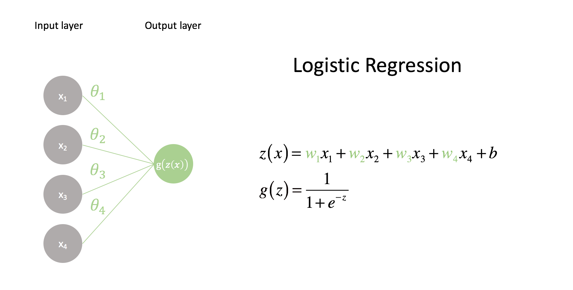
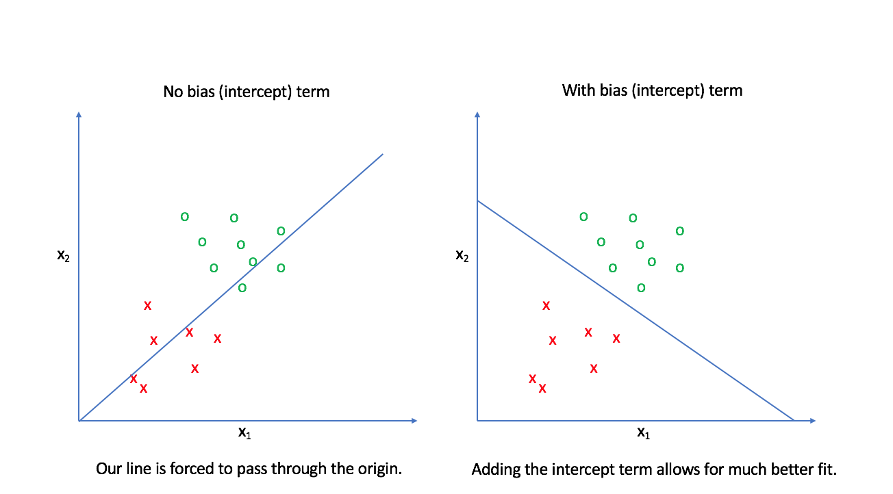
The first layer contains a node for each value in our input feature vector. These values are scaled by their corresponding weight, $w_i$, and added together along with a bias term, $b$. The bias term allows us to build linear models that aren't fixed at the origin. The following image provides an example of why this is important. Notice how we can provide a much better decision boundary for logistic regression when our linear model isn't fixed at the origin.
The input nodes in our network visualization are all connected to a single output node, which consists of a linear combination of all of the inputs. Each connection between nodes contains a parameter, $w$, which is what we'll tune to form an optimal model (tuning these parameters will be covered in a later post). The final output is functional composition, $g\left( {z\left( x \right)} \right)$. When we pass the linear combination of inputs through the logistic (also known as sigmoid) function, the neural network community refers to this as activation. Namely, the sigmoid is an activation function which controls whether or not the end node "neuron" will fire. As you'll see later, there's a whole family of possible activation functions that we can use.
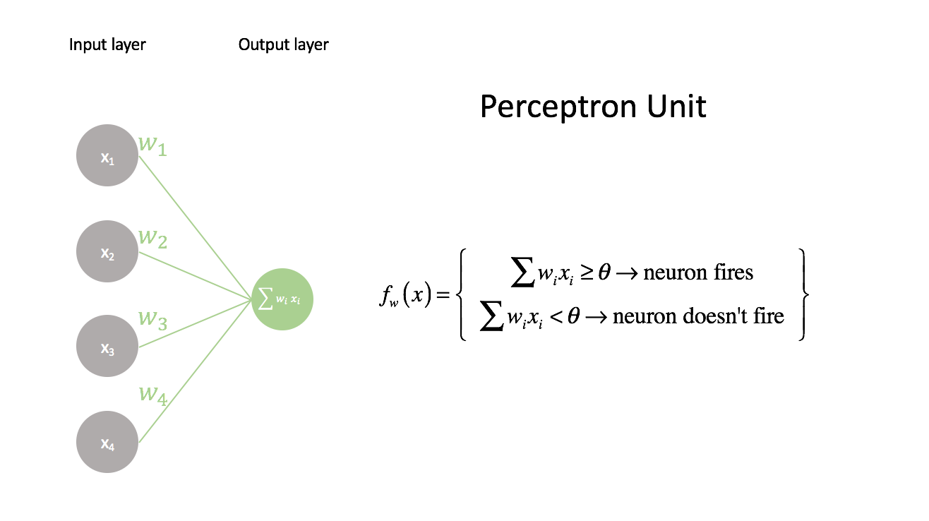
Comparison to a perceptron unit
Most tutorials will introduce the concept of a neural network with the perceptron, but I've found it's easier to introduce the concept of neural networks by latching onto something familiar (logistic regression). However, for the sake of completeness I'll go ahead and introduce the perceptron unit and note its similarities to the network representation of logistic regression.
The perceptron is the simplest neural unit that we can build. It takes a series of inputs, $x_i$, combined with a series of weights, $w_i$, which are compared against a threshold value, $\theta$. If the linear combination of inputs and weights is higher than the threshold, the neuron fires, and if the combination is less than the threshold it doesn't fire.
We can rewrite the perceptron function by moving the threshold to the left side and we end up with the same linear model used in logistic regression. The weights, $w_i$ in the perceptron algorithm are synonomous with the weights in logistic regression and the threshold value, $\theta$, in the perceptron algorithm is synonomous with bias $b$.
At a high level, they're practically identical - the main difference being the activation function, $g\left( z \right)$, used to control neuron firing. The perceptron activation is a step-function from 0 (when the neuron doesn't fire) to 1 (when the neuron fires) while the logistic regression model has a smoother activation function with values ranging from 0 to 1.
Building a network of neurons
The previous model is only capable of binary classification; however, recall that we can perform multi-class classification by building a collection of logistic regression models. Let's extend our "network" to represent this.
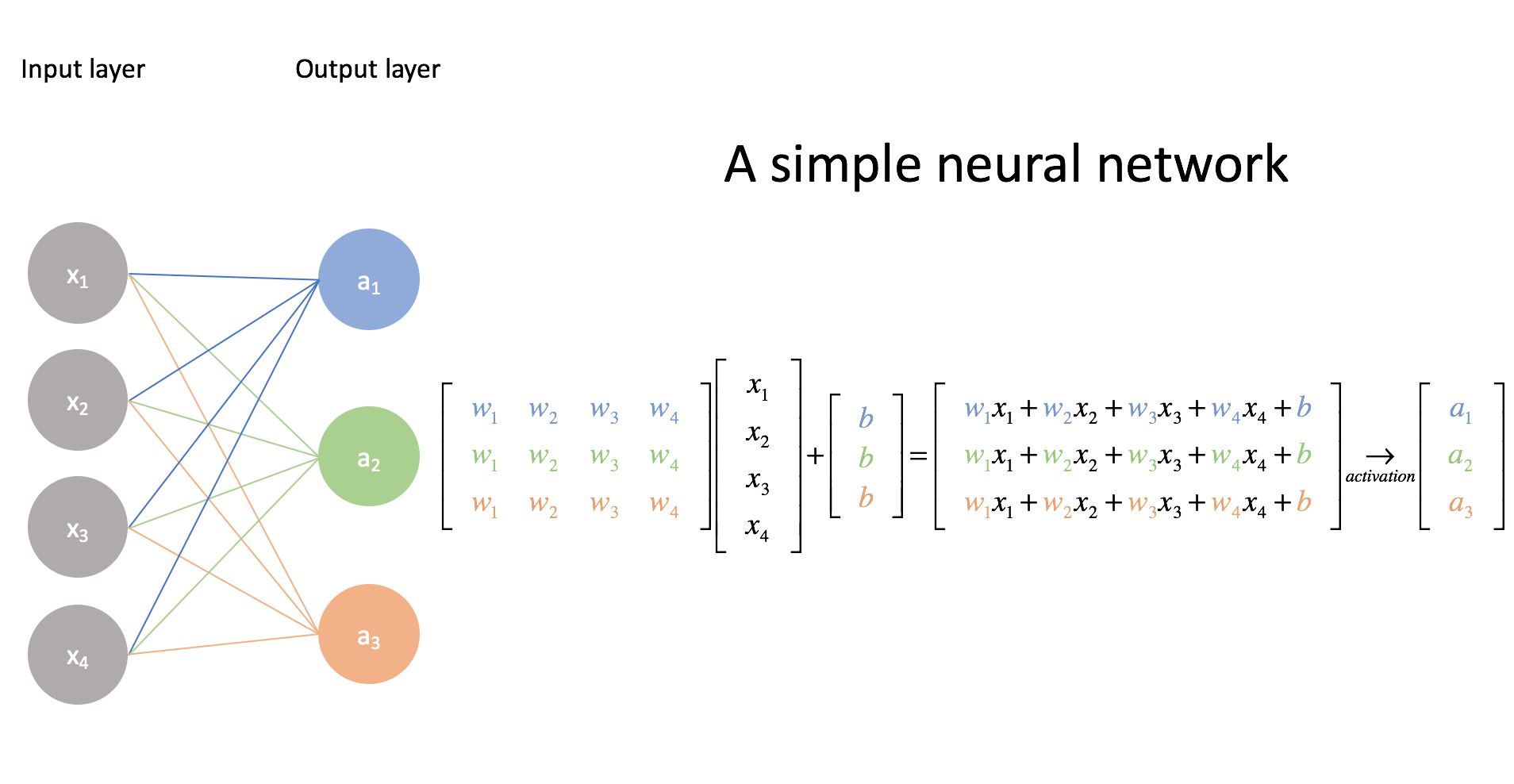
Note: While I didn't explicitly show the activation function here, we still use it on each linear combination of inputs. I mainly just wanted to show the connection between the visual representation and matrix form.
Here, we've built three distinct logistic regression models, each with their own set of parameters. Take a moment to make sure you understand this matrix representation. (This is why matrix multiplication is listed as a prerequisite.) It's rather convenient that we can leverage matrix operations as it allows us to perform these calculations quickly and efficiently.
The above example displays the case for multi-class classification on a single example, but we can also extend our input matrix to classify a collection of examples. This is not simply useful, but necessary for our optimization algorithm (in a later post) to learn from all of the examples in an efficient manner when finding the best parameters (more commonly referred to as weights in the neural network community).
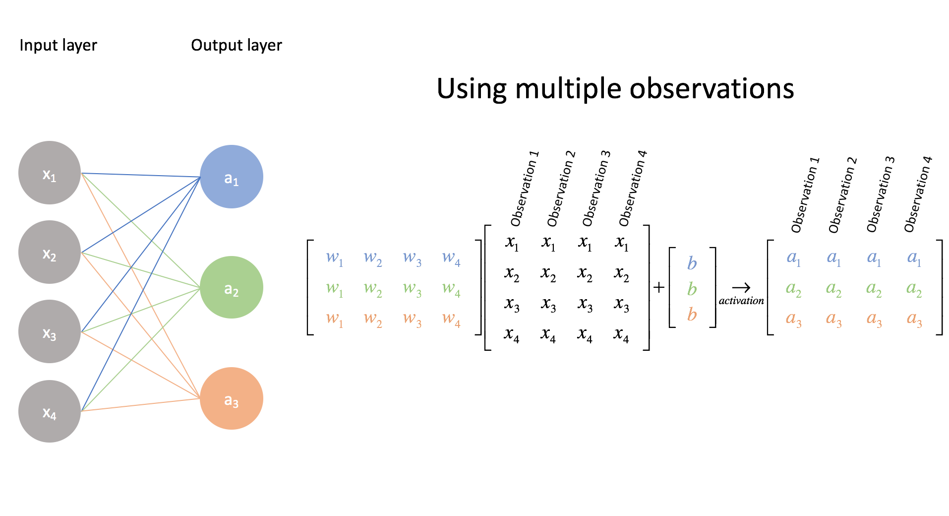
Again, go through the matrix multiplications to convince yourself of this.
Although I color coded the weights here for clarity, we'll need to develop a more systematic notation. Notice how the first output neuron uses all of the blue weights, the second output neuron uses all of the green weights, and the third output neuron uses all of the orange weights.
Moving forward, we'll describe our weights more succinctly as a vector $w_i$ where the subscript $i$ now represents the neuron which uses that set of weights.
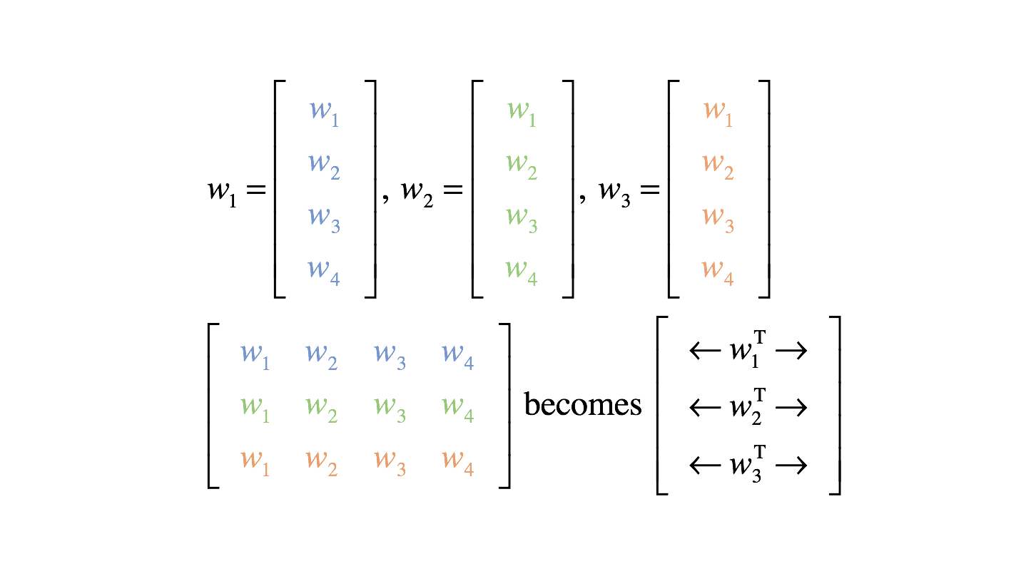
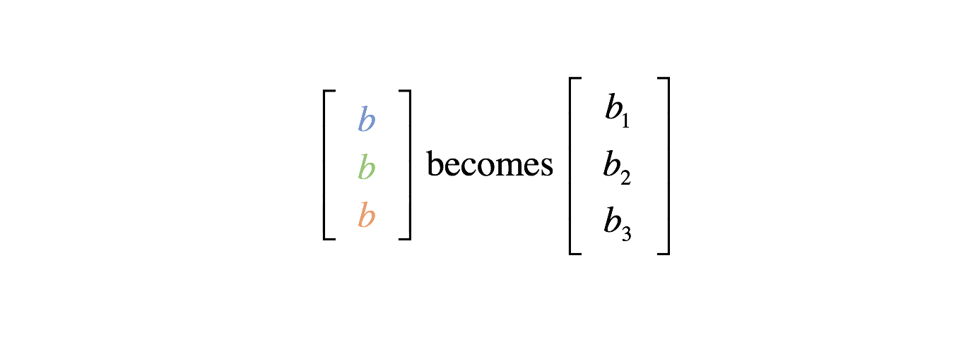
Thus, we can define a weight matrix, $W$, for a layer. Our bias may similarly be described as a vector $b$.
Hidden layers
Up until now, we've been dealing solely with one-layer networks; we feed information into the input layer and observe the results in the output layer. (The input layer often isn't counted as a layer in the neural network.)
The real power of neural networks emerges as we add additional layers to the network. Any layer that is between the input and output layers is known as a hidden layer. Thus, the following example is a neural network with an input layer, one hidden layer, and an output layer.
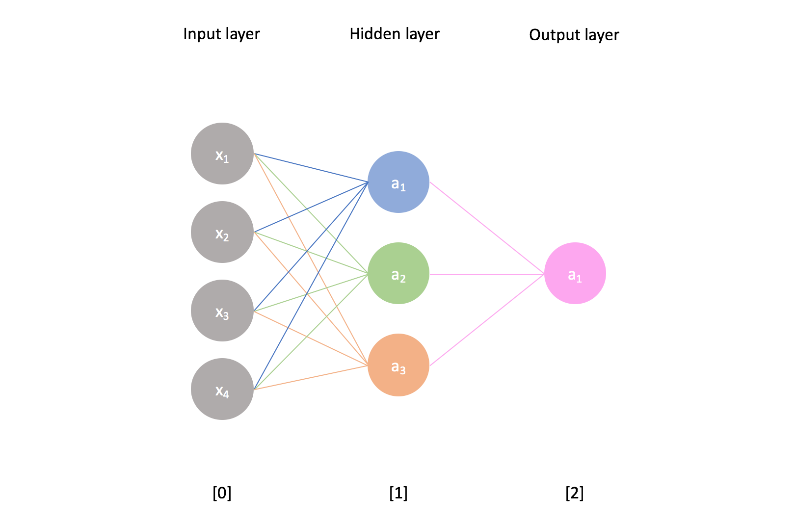
I'll use the superscript $\left[ l \right]$ to refer to the ${l^{th}}$ layer of the network and the subscript $i$ to refer to the ${i^{th}}$ neuron in a layer.
For example, $a_2^{\left[ 1 \right]}$ represents the activation of the second neuron in the first hidden layer. We can calculate this value by first combining the proper weights and bias with the previous layer's values
$$ z_2^{\left[ 1 \right]} = w_2^{\left[ 1 \right]{\rm{T}}}{a^{\left[ 0 \right]}} + {b_2} $$
and then passing this through our activation function, $g\left( z \right)$. Notice how each neuron combines every value from the previous layer as input.
Note: Our input vector, $x$, can also be referred to as the activations of the $0^{th}$ layer.
More generally, we can calculate the activation of neuron $i$ in layer $l$.
$$ z_i^{\left[ l \right]} = w_i^{\left[ l \right]{\rm{T}}}{a^{\left[ {l - 1} \right]}} + b_i^{\left[ l \right]} $$
$$ a_i^{\left[ l \right]} = g\left( {z_i^{\left[ l \right]}} \right) $$
Similarly, we can calculate all of the activations for a given layer $l$ by using our weight matrix ${W^{\left[ l \right]}}$.
$$ {Z^{\left[ l \right]}} = {W^{\left[ l \right]}}{A^{\left[ {l - 1} \right]}} + {b^{\left[ l \right]}} $$
$$ {A^{\left[ l \right]}} = g\left( {{Z^{\left[ l \right]}}} \right) $$
In a network, we take the output from one layer and feed it in as the input to our next layer. We can stack as many layers as we want on top of each other. The field of deep learning studies neural network architectures with many hidden layers.
Matrix representation
Let ${n^{\left[ l \right]}}$ represent the number of units in layer $l$. For a given layer, we'll have a weights matrix ${W^{\left[ l \right]}}$ of shape $\left( {{n^{\left[ l \right]}},{n^{\left[ {l - 1} \right]}}} \right)$ and a bias vector of shape $\left( {{n^{\left[ l \right]}},1} \right)$.
The activations of a given layer will be a matrix of shape $\left( {{n^{\left[ l \right]}},m} \right)$ where $m$ represents the number of observations being fed through the network. Recall the earlier section where I demonstrated calculating the neural network output of multiple observations using an efficient matrix representation.
When I was first learning about neural networks, the trickiest part for me was figuring out what my matrix dimensions needed to be and how to manipulate them to get them into the proper form. I'd recommend doing a couple practice problems to get more comfortable before we continue to talk about training a neural network in my next post.
Feeling like you've got a grasp? Check out this neural network cheat sheet of common architectures.