Neural networks: training with backpropagation.

In my first post on neural networks, I discussed a model representation for neural networks and how we can feed in inputs and calculate an output. We calculated this output, layer by layer, by combining the inputs from the previous layer with weights for each neuron-neuron connection. I mentioned that we'd talk about how to find the proper weights to connect neurons together in a future post - this is that post!

Overview

In the previous post I had just assumed that we had magic prior knowledge of the proper weights for each neural network. In this post, we'll actually figure out how to get our neural network to "learn" the proper weights. However, for the sake of having somewhere to start, let's just initialize each of the weights with random values as an initial guess. We'll come back and revisit this random initialization step later on in the post.

Given our randomly initialized weights connecting each of the neurons, we can now feed in our matrix of observations and calculate the outputs of our neural network. This is called forward propagation. Given that we chose our weights at random, our output is probably not going to be very good with respect to our expected output for the dataset.

So where do we go from here?

Well, for starters, let's define what a "good" output looks like. Namely, we'll develop a cost function which penalizes outputs far from the expected value.

Next, we need to figure out a way to change the weights so that the cost function improves. Any given path from an input neuron to an output neuron is essentially just a composition of functions; as such, we can use partial derivatives and the chain rule to define the relationship between any given weight and the cost function. We can use this knowledge to then leverage gradient descent in updating each of the weights.

Pre-requisites

When I was first learning backpropagation, many people tried to abstract away the underlying math (derivative chains) and I was never really able to grasp what the heck was going on until watching Professor Winston's lecture at MIT. I hope that this post gives a better understanding of backpropagation than simply "this is the step where we send the error backwards to update the weights".

In order to fully grasp the concepts discussed in this post, you should be familiar with the following:

Partial derivatives
This post is going to be a bit dense with a lot of partial derivatives. However, it is my hope that even a reader without prior knowledge of multivariate calculus can still follow the logic behind backpropagation.

If you're not familiar with calculus, $\frac{{\partial f\left( x \right)}}{{\partial x}}$ will probably look pretty foreign. You can interpret this expression as "how does $f\left( x \right)$ change as I change $x$?" This will be useful because we can ask questions like "How does the cost function change when I change this parameter? Does it increase or decrease the cost function?" in search of the optimal parameters.

If you'd like to brush up on multivariate calculus, check out Khan Academy's lessons on the subject.

Gradient descent
To prevent this post from getting too long, I've separated the topic of gradient descent into another post. If you're not familiar with the method, be sure to read about it here and understand it before continuing this post.

Matrix multiplication
Here is a quick refresher from Khan Academy.

Starting simple

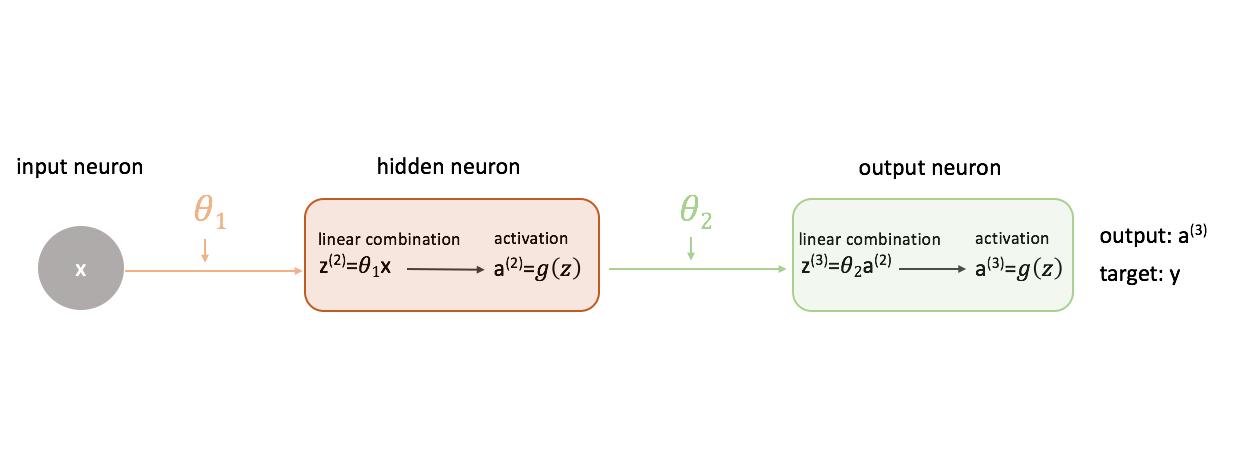
To figure out how to use gradient descent in training a neural network, let's start with the simplest neural network: one input neuron, one hidden layer neuron, and one output neuron.

To show a more complete picture of what's going on, I've expanded each neuron to show 1) the linear combination of inputs and weights and 2) the activation of this linear combination. It's easy to see that the forward propagation step is simply a series of functions where the output of one feeds as the input to the next.

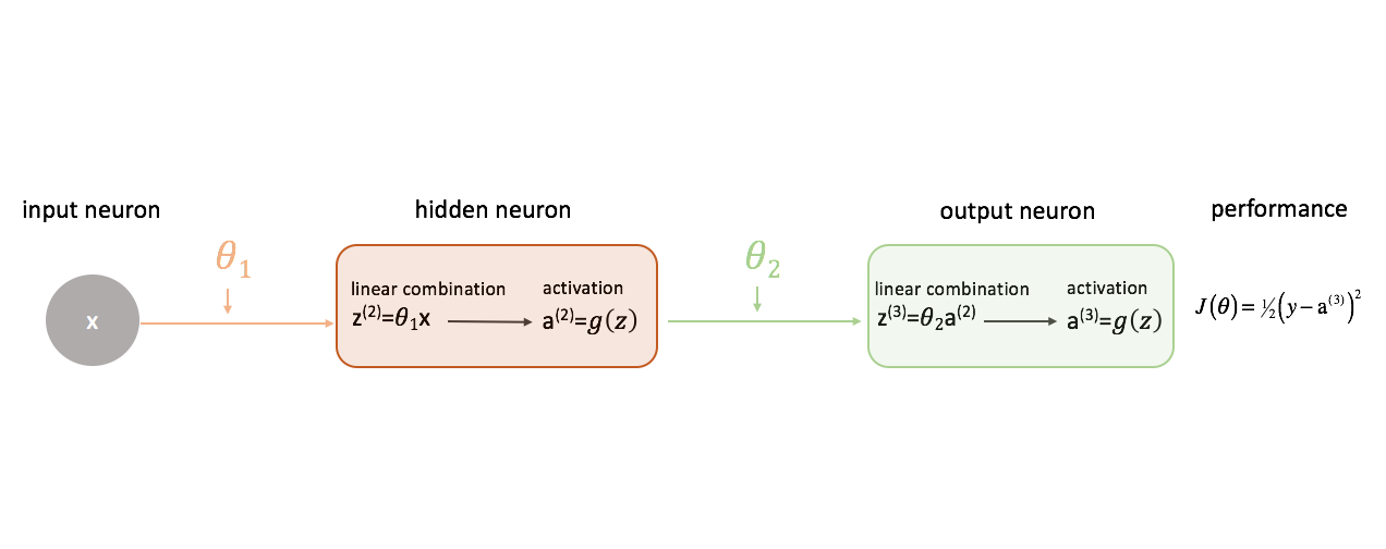
Defining "good" performance in a neural network

Let's define our cost function to simply be the squared error.

[J\left( \theta \right) = {\raise0.5ex\hbox{$\scriptstyle 1$}
\kern-0.1em/\kern-0.15em
\lower0.25ex\hbox{$\scriptstyle 2$}}{\left( {y - {{\rm{a}}^{(3)}}} \right)^2}]

There's a myriad of cost functions we could use, but for this neural network squared error will work just fine.

Remember, we want to evaluate our model's output with respect to the target output in an attempt to minimize the difference between the two.

Relating the weights to the cost function

In order to minimize the difference between our neural network's output and the target output, we need to know how the model performance changes with respect to each parameter in our model. In other words, we need to define the relationship (read: partial derivative) between our cost function and each weight. We can then update these weights in an iterative process using gradient descent.

[\frac{{\partial J\left( \theta \right)}}{{\partial {\theta _1}}} = ?]

[\frac{{\partial J\left( \theta \right)}}{{\partial {\theta _2}}} = ?]

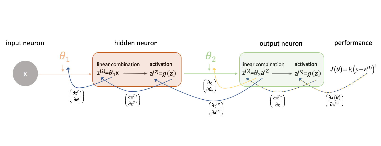
Let's look at $\frac{{\partial J\left( \theta \right)}}{{\partial {\theta _2}}}$ first. Keep the following figure in mind as we progress.

Let's take a moment to examine how we could express the relationship between $J\left( \theta \right)$ and $\theta _2$. Note how $\theta _2$ is an input to ${z^{(3)}}$, which is an input to ${{\rm{a}}^{(3)}}$, which is an input to $J\left( \theta \right)$. When we're trying to compute a derivative of this sort, we can use the chain rule to solve.

As a reminder, the chain rule states:
[\frac{\partial }{{\partial z}}p\left( {q\left( z \right)} \right) = \frac{{\partial p}}{{\partial q}}\frac{{\partial q}}{{\partial z}}]

Let's apply the chain rule to solve for $\frac{{\partial J\left( \theta \right)}}{{\partial {\theta _2}}}$.

[\frac{{\partial J\left( \theta \right)}}{{\partial {\theta _2}}} = \left( {\frac{{\partial J\left( \theta \right)}}{{\partial {{\rm{a}}^{(3)}}}}} \right)\left( {\frac{{\partial {{\rm{a}}^{(3)}}}}{{\partial z}}} \right)\left( {\frac{{\partial z}}{{\partial {\theta _2}}}} \right)]

By similar logic, we can find $\frac{{\partial J\left( \theta \right)}}{{\partial {\theta _1}}}$.

[\frac{{\partial J\left( \theta \right)}}{{\partial {\theta _1}}} = \left( {\frac{{\partial J\left( \theta \right)}}{{\partial {{\rm{a}}^{(3)}}}}} \right)\left( {\frac{{\partial {{\rm{a}}^{(3)}}}}{{\partial {z^{(3)}}}}} \right)\left( {\frac{{\partial {z^{(3)}}}}{{\partial {{\rm{a}}^{(2)}}}}} \right)\left( {\frac{{\partial {{\rm{a}}^{(2)}}}}{{\partial {z^{(2)}}}}} \right)\left( {\frac{{\partial {z^{(2)}}}}{{\partial {\theta _1}}}} \right)]

For the sake of clarity, I've updated our neural network diagram to visualize these chains. Make sure you are comfortable with this process before proceeding.

Adding complexity

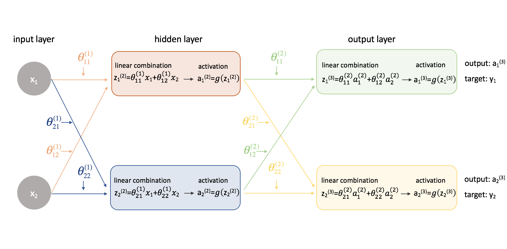
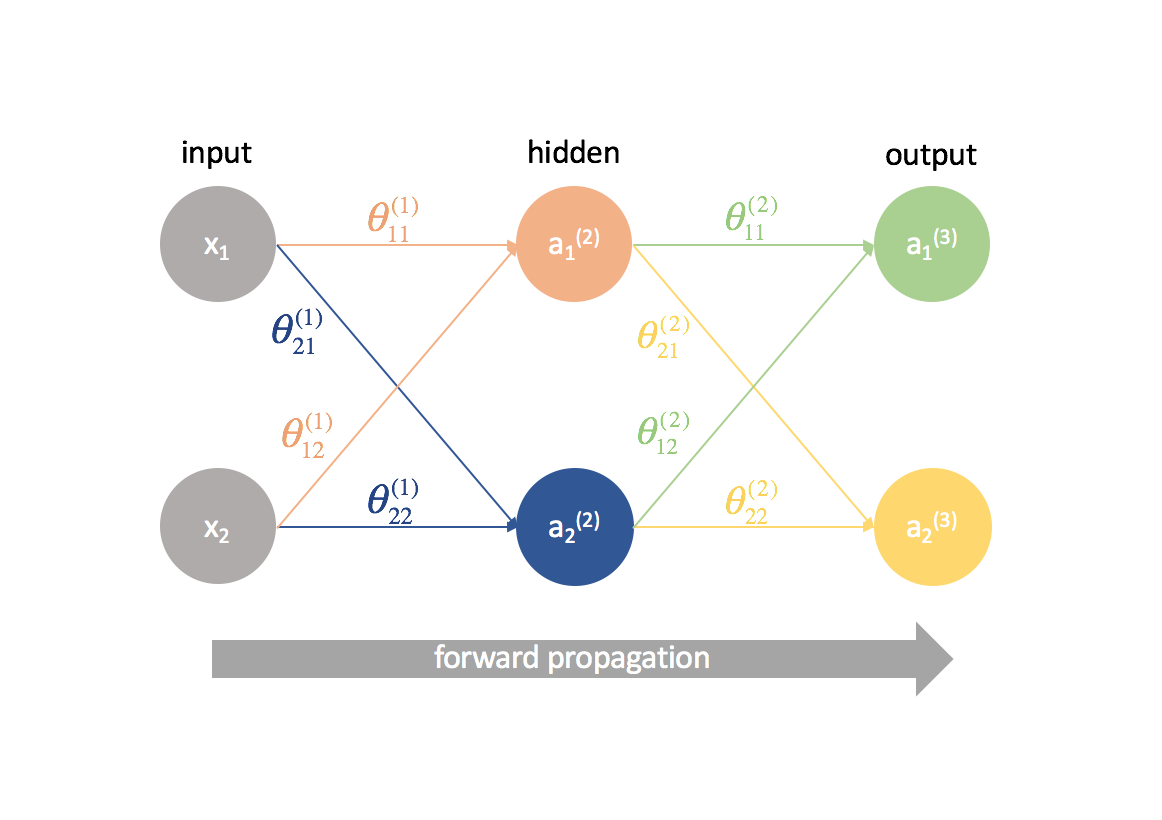
Now let's try this same approach on a slightly more complicated example. Now, we'll look at a neural network with two neurons in our input layer, two neurons in one hidden layer, and two neurons in our output layer. For now, we'll disregard the bias neurons that are missing from the input and hidden layers.

Let's take a second to go over the notation I'll be using so you can follow along with these diagrams. The superscript ⁽¹⁾ denotes what layer the object is in and the subscript denotes which neuron we're referring to in a given layer. For example $a_1^{(2)}$ is the activation of the first neuron in the second layer. For the parameter values $\theta$, I like to read them like a mailing label - the first value denotes what neuron the input is being sent to in the next layer, and the second value denotes from what neuron the information is being sent. For example, ${\theta _{21}^{(2)}}$ is used to send input to the 2^nd neuron, from the 1^st neuron in layer 2. The superscript denoting the layer corresponds with where the input is coming from. This notation is consistent with the matrix representation we discussed in my post on neural networks representation.

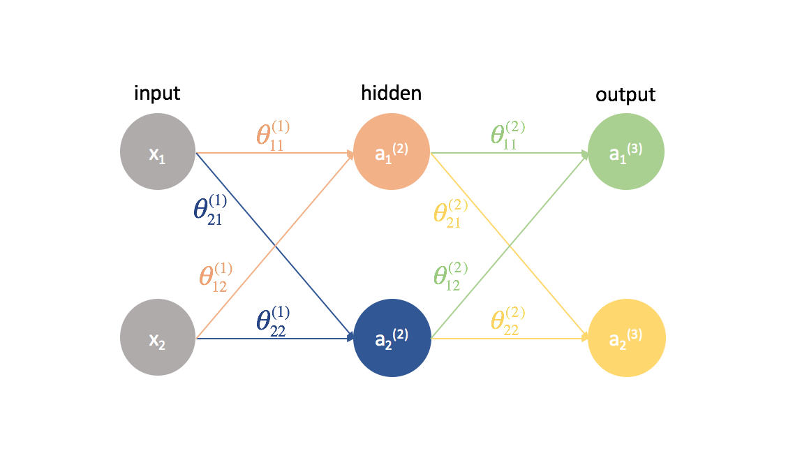
Let's expand this network to expose all of the math that's going on.

Yikes! Things got a little more complicated. I'll walk through the process for finding one of the partial derivatives of the cost function with respect to one of the parameter values; I'll leave the rest of the calculations as an exercise for the reader (and post the end results below).

Foremost, we'll need to revisit our cost function now that we're dealing with a neural network with more than one output. Let's now use the mean squared error as our cost function.

[J\left( \theta \right) = \frac{1}{{2m}}\sum{{{\left( {{y _i} - {\rm{a}} _i^{(2)}} \right)}^2}} ]

Note: If you're training on multiple observations (which you always will in practice), we'll also need to perform a summation of the cost function over all training examples. For this cost function, it's common to normalize by $\frac{1}{{m}}$ where $m$ is the number of examples in your training dataset.

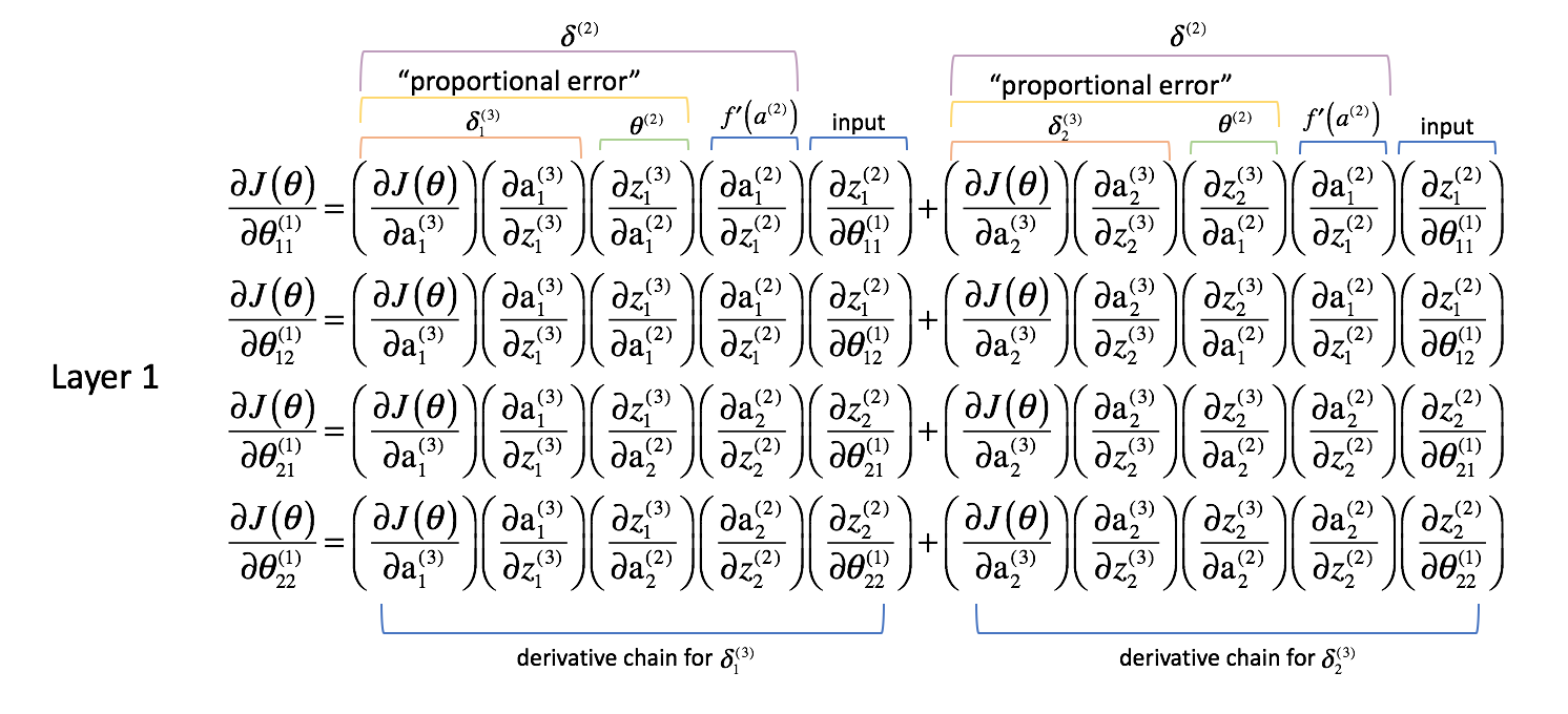
Now that we've corrected our cost function, we can look at how changing a parameter affects the cost function. Specifically, I'll calculate $\frac{{\partial J\left( \theta \right)}}{{\partial \theta _{11}^{(1)}}}$ in this example. Looking at the diagram, $\theta _{11}^{(1)}$ affects the output for both $a _1^{(3)}$ and $a _2^{(3)}$. Because our cost function is a summation of individual costs for each output, we can calculate the derivative chain for each path and simply add them together.

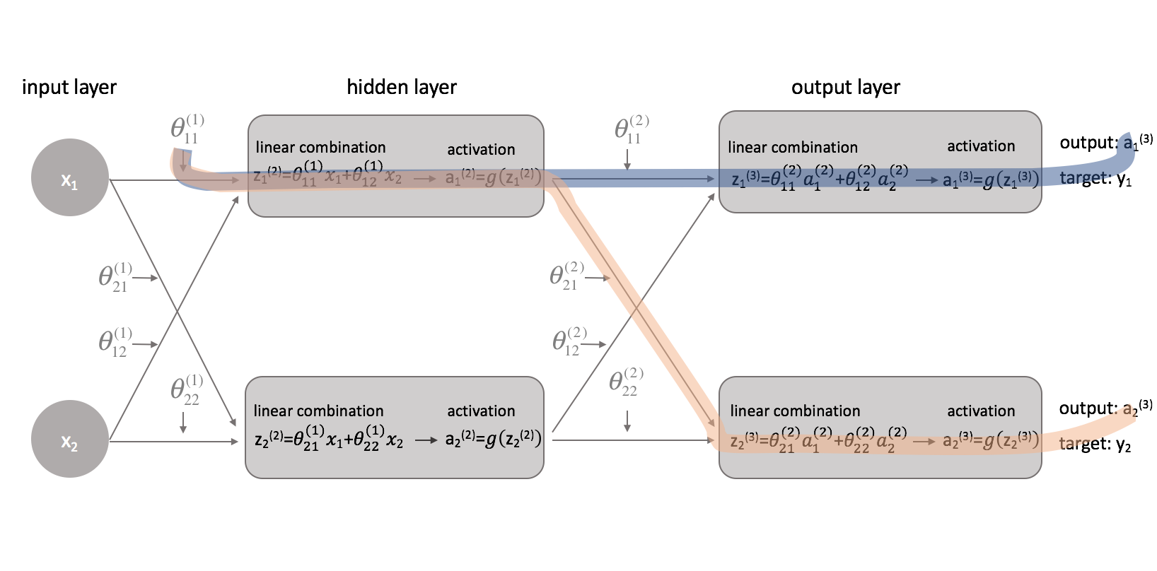
The derivative chain for the blue path is:
$$ \left( {\frac{{\partial J\left( \theta \right)}}{{\partial {\rm{a}} _1^{(3)}}}} \right)\left( {\frac{{\partial {\rm{a}} _1^{(3)}}}{{\partial z _1^{(3)}}}} \right)\left( {\frac{{\partial z _1^{(3)}}}{{\partial {\rm{a}} _1^{(2)}}}} \right)\left( {\frac{{\partial {\rm{a}} _1^{(2)}}}{{\partial z _1^{(2)}}}} \right)\left( {\frac{{\partial z _1^{(2)}}}{{\partial \theta _{11}^{(1)}}}} \right) $$

The derivative chain for the orange path is:
$$ \left( {\frac{{\partial J\left( \theta \right)}}{{\partial {\rm{a}} _2^{(3)}}}} \right)\left( {\frac{{\partial {\rm{a}} _2^{(3)}}}{{\partial z _2^{(3)}}}} \right)\left( {\frac{{\partial z _2^{(3)}}}{{\partial {\rm{a}} _1^{(2)}}}} \right)\left( {\frac{{\partial {\rm{a}} _1^{(2)}}}{{\partial z _1^{(2)}}}} \right)\left( {\frac{{\partial z _1^{(2)}}}{{\partial \theta _{11}^{(1)}}}} \right)$$

Combining these, we get the total expression for $\frac{{\partial J\left( \theta \right)}}{{\partial \theta _{11}^{(1)}}}$.

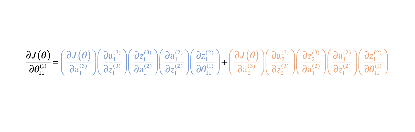
I've provided the remainder of the partial derivatives below. Remember, we need these partial derivatives because they describe how changing each parameter affects the cost function. Thus, we can use this knowledge to change all of the parameter values in a way that continues to decrease the cost function until we converge on some minimum value.

Layer 2 Parameters

Layer 1 Parameters

Woah there. We just went from a neural network with 2 parameters that needed 8 partial derivative terms in the previous example to a neural network with 8 parameters that needed 52 partial derivative terms. This is going to quickly get out of hand, especially considering many neural networks that are used in practice are much larger than these examples.

Fortunately, upon closer inspection many of these partial derivatives are repeated. If we're smart about how we approach this problem, we can dramatically reduce the computational cost of training. Further, it'd really be a pain in the ass if we had to manually calculate the derivative chains for every parameter. Let's look at what we've done so far and see if we can generalize a method to this madness.

Generalizing a method

Let's examine the partial derivatives above and make a few observations. We'll start with looking at the partial derivatives with respect to the parameters for layer 2. Remember, the parameters in for layer 2 are combined with the activations in layer 2 to feed as inputs into layer 3.

Layer 2 Parameters

Let's analyze the following expressions; I encourage you to solve the partial derivatives as we go along to convince yourself of my logic.

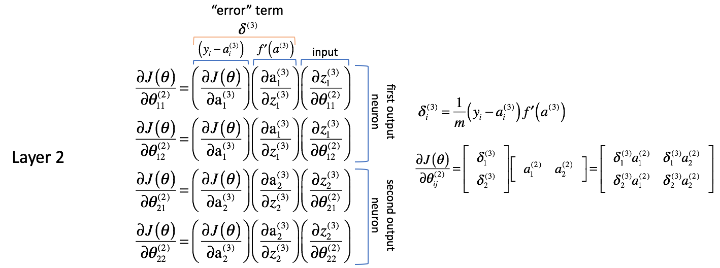
Foremost, it seems as if the columns contain very similar values. For example, the first column contains partial derivatives of the cost function with respect to the neural network outputs. In practice, this is the difference between the expected output and the actual output (and then scaled by $m$) for each of the output neurons.

The second column represents the derivative of the activation function used in the output layer. Note that for each layer, neurons will use the same activation function. A homogenous activation function within a layer is necessary in order to be able to leverage matrix operations in calculating the neural network output. Thus, the value for the second column will be the same for all four terms.

The first and second columns can be combined as $\delta _i^{(3)}$ for the sake of convenience later on down the road. It is not immediately evident why this would be helpful, but you'll see as we go backwards another layer why this is useful. People will often refer to this expression as the "error" term which we use to "send back error from the output throughout the network". We'll see why this is the case soon. Each neuron in the network will have a corresponding $\delta$ term that we'll solve for.

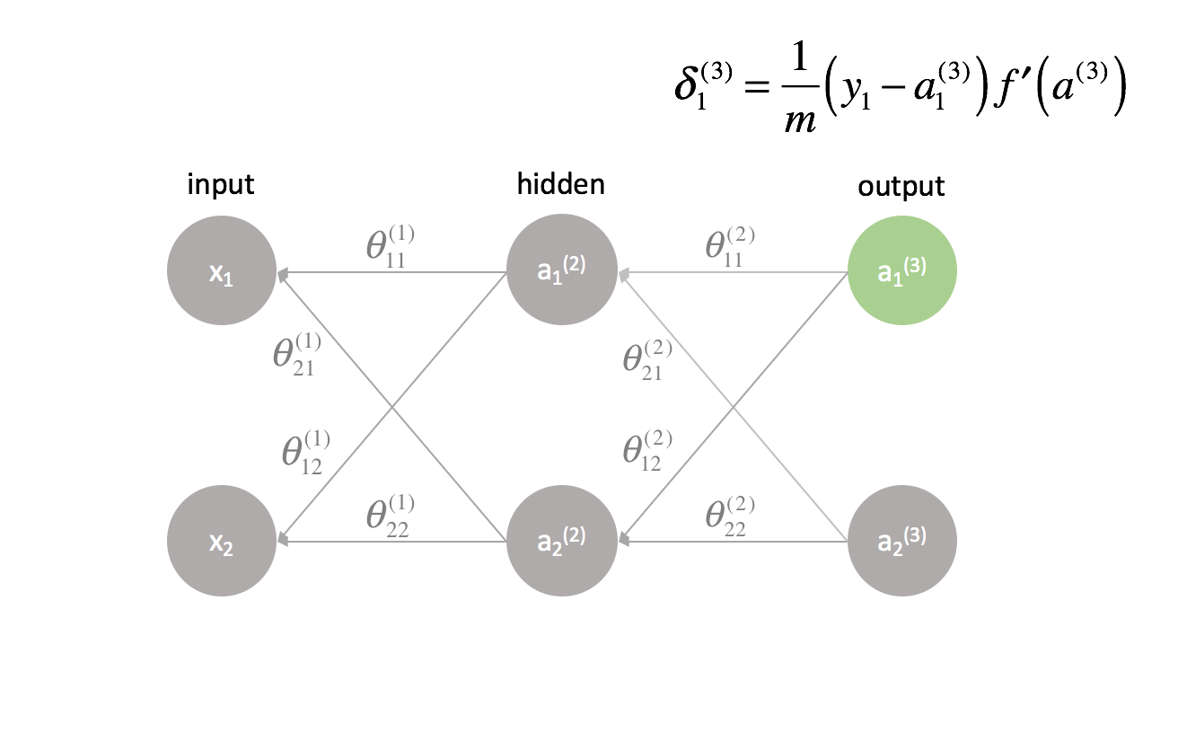
[\delta _i^{(3)} = \frac{1}{m}\left( {{y _i} - a _i^{(3)}} \right)f'\left( {{a^{(3)}}} \right)]

The third column represents how the parameter of interest changes with respect to the weighted inputs for the current layer; when you calculate the derivative this corresponds with the activation from the previous layer.

I'd also like to note that the first two partial derivative terms seem concerned with the first output neuron (neuron 1 in layer 3) while the last two partial derivative terms seem concerned with the second output neuron (neuron 2 in layer 3). This is evident in the $\frac{{\partial J\left( \theta \right)}}{{\partial {\rm{a}}_i^{(3)}}}$ term. Let's use this knowledge to rewrite the partial derivatives using the $\delta$ expression we defined above.

Next, let's go ahead and calculate the last partial derivative term. As we noted, this partial derivative ends up representing activations from the previous layer.

Note: I find it helpful to use the expanded neural network graphic in the previous section when calculating the partial derivatives.

It appears that we're combining the "error" terms with activations from the previous layer to calculate each partial derivative. It's also interesting to note that the indices $j$ and $k$ for $\theta _{jk}$ match the combined indices of $\delta _j^{(3)}$ and ${\rm{a}} _k^{(2)}$.

[\frac{{\partial J\left( \theta \right)}}{{\partial \theta _{jk}^{(2)}}} = \delta _j^{(3)}{\rm{a}} _k^{(2)}]

Let's see if we can figure out a matrix operation to compute all of the partial derivatives in one expression.

${\delta ^{(3)}}$ is a vector of length $j$ where $j$ is equal to the number of output neurons.

${\rm{a}}^{(2)}$ is a vector of length $k$ where $k$ is the number of neurons in the previous layer. The values of this vector represent activations of the previous layer calculated during forward propagation; in other words, it's the vector of inputs to the output layer.

$$ {a^{(2)}} = \left[ {\begin{array}{* {20}{c}}
{a _1^{(2)}}&{a _2^{(2)}}& \cdots &{a _k^{(2)}}
\end{array}} \right] $$

Multiplying these vectors together, we can calculate all of the partial derivative terms in one expression.

To summarize, see the graphic below.

Note: Technically, the first column should also be scaled by $m$ to be an accurate derivative. However, my focus was to point out that this is the column where we're concerned with the difference between the expected and actual outputs. The $\delta$ term on the right has the full derivative expression.

Layer 1 Parameters

Now let's take a look and see what's going on in layer 1.

Whereas the weights in layer 2 only directly affected one output, the weights in layer 1 affect all of the outputs. Recall the following graphic.

This results in a partial derivative of the cost function with respect to a parameter now becoming a summation of different chains. Specifically, we'll have a derivative chain for every $\delta$ we calculated in the next layer forward. Remember, we started at the end of the network and are working our way backwards through the network. Thus, the next layer forward represents the $\delta$ values that we previously calculated.

As we did for layer 2, let's make a few observations.

The first two columns (of each summed term) corresponds with a $\delta _j^{(3)}$ calculated in the next layer forward (remember, we started at the end of the network and are working our way back).

The third column corresponds with some parameter that connects layer 2 to layer 3. If we considered $\delta _j^{(3)}$ to be some "error" term for layer 3, and each derivative chain is now a summation of these errors, then this third column allows us to weight each respective error. Thus, the first three terms combined represent some measure of the proportional error.

We'll also redefine $\delta$ for all layers excluding the output layer to include this combination of weighted errors.

$$ \delta _j^{(l)} = f'\left( {{a^{(l)}}} \right)\sum\limits _{i = 1}^n {\delta _i^{(l + 1)}\theta _{ij}^{(l)}} $$

We could write this more succinctly using matrix expressions.

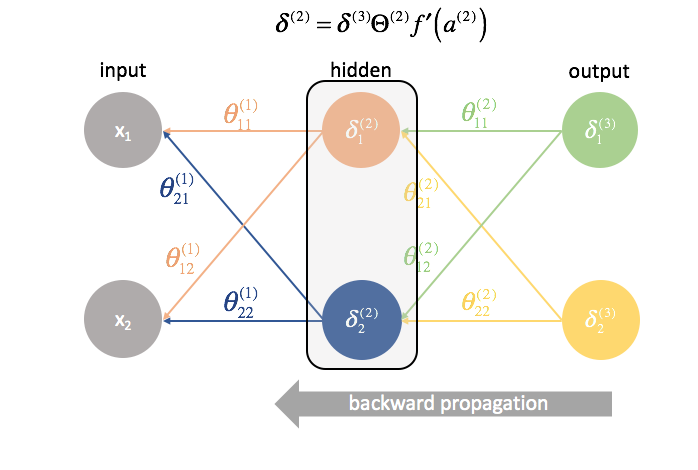
$$ {\delta ^{(l)}} = {\delta ^{(l + 1)}}{\Theta ^{(l)}}f'\left( {{a^{(l)}}} \right) $$

Note: It's standard notation to denote vectors with lowercase letters and matrices as uppercase letters. Thus, $\theta$ represents a vector while $\Theta$ represents a matrix.

The fourth column represents the derivative of the activation function used in the current layer. Remember that for each layer, neurons will use the same activation function.

Lastly, the fifth column represents various inputs from the previous layer. In this case, it is the actual inputs to the neural network.

Let's take a closer look at one of the terms, $\frac{{\partial J\left( \theta \right)}}{{\partial \theta _{11}^{(1)}}}$.

Foremost, we established that the first two columns of each derivative chains were previously calculated as $\delta _j^{(3)}$.

$$ \frac{{\partial J\left( \theta \right)}}{{\partial \theta _{11}^{(1)}}} = \delta _1^{(3)}\left( {\frac{{\partial z _1^{(3)}}}{{\partial {\rm{a}} _1^{(2)}}}} \right)\left( {\frac{{\partial {\rm{a}} _1^{(2)}}}{{\partial z _1^{(2)}}}} \right)\left( {\frac{{\partial z _1^{(2)}}}{{\partial \theta _{11}^{(1)}}}} \right) + \delta _2^{(3)}\left( {\frac{{\partial z _2^{(3)}}}{{\partial {\rm{a}} _1^{(2)}}}} \right)\left( {\frac{{\partial {\rm{a}} _1^{(2)}}}{{\partial z _1^{(2)}}}} \right)\left( {\frac{{\partial z _1^{(2)}}}{{\partial \theta _{11}^{(1)}}}} \right) $$

Further, we established the the third columns of each derivative chain was a parameter that acted to weight each of the respective $\delta$ terms. We also established that the fourth column was the derivative of the activation function.

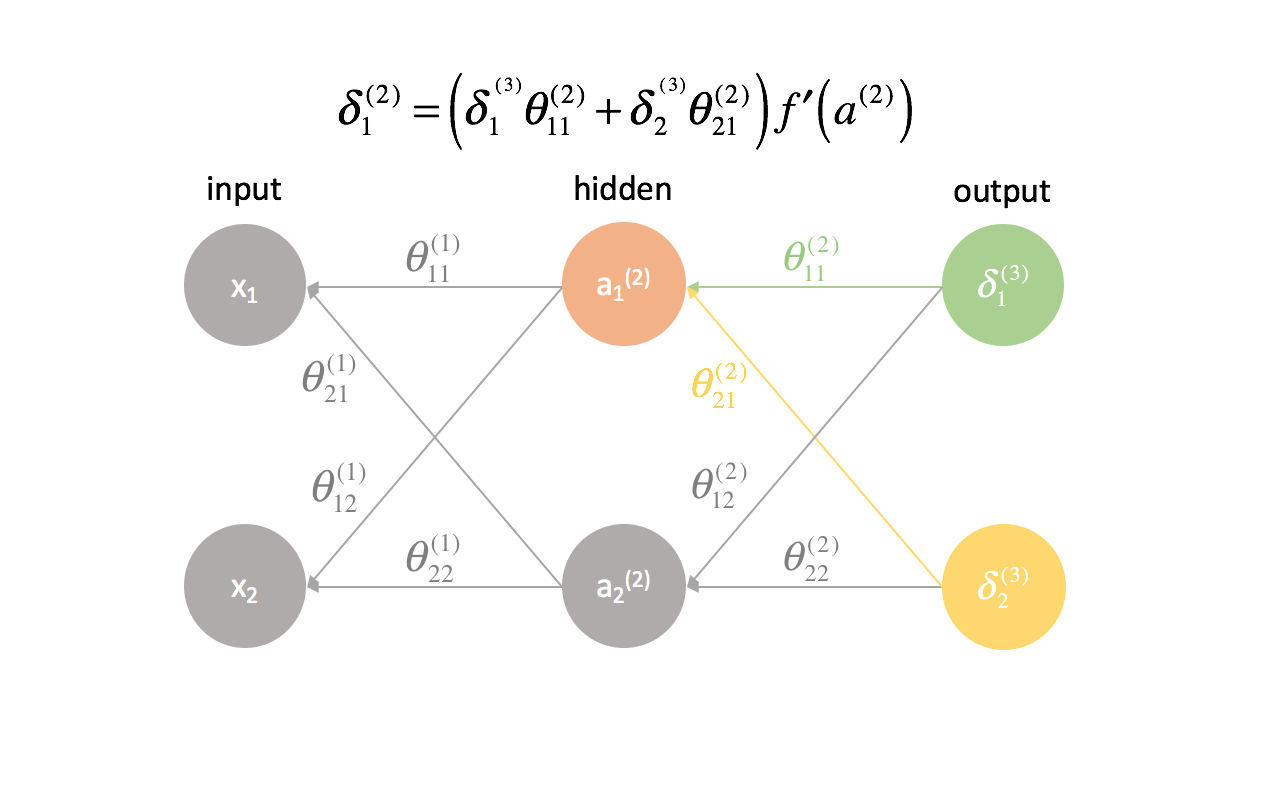
$$ \frac{{\partial J\left( \theta \right)}}{{\partial \theta _{11}^{(1)}}} = \delta _1^{(3)}\theta _{11}^{(2)}f'\left( {{a^{(2)}}} \right)\left( {\frac{{\partial z _1^{(2)}}}{{\partial \theta _{11}^{(1)}}}} \right) + \delta _2^{(3)}\theta _{21}^{(2)}f'\left( {{a^{(2)}}} \right)\left( {\frac{{\partial z _1^{(2)}}}{{\partial \theta _{11}^{(1)}}}} \right) $$

Factoring out $\left( {\frac{{\partial z_1^{(2)}}}{{\partial \theta _{11}^{(1)}}}} \right)$,

$$ \frac{{\partial J\left( \theta \right)}}{{\partial \theta _{11}^{(1)}}} = \left( {\frac{{\partial z _1^{(2)}}}{{\partial \theta _{11}^{(1)}}}} \right)\left( {\delta _1^{(3)}\theta _{11}^{(2)}f'\left( {{a^{(2)}}} \right) + \delta _2^{(3)}\theta _{21}^{(2)}f'\left( {{a^{(2)}}} \right)} \right) $$

we're left with our new definition of $\delta_j^{(l)}$. Let's go ahead and substitute that in.

$$ \frac{{\partial J\left( \theta \right)}}{{\partial \theta _{11}^{(1)}}} = \left( {\frac{{\partial z _1^{(2)}}}{{\partial \theta _{11}^{(1)}}}} \right)\left( {\delta _1^{(2)}} \right) $$

Lastly, we established the fifth column (${\frac{{\partial z_1^{(2)}}}{{\partial \theta_{11}^{(1)}}}}$) corresponded with an input from the previous layer. In this case, the derivative calculates to be $x_1$.

$$ \frac{{\partial J\left( \theta \right)}}{{\partial \theta _{11}^{(1)}}} = \delta _1^{(2)}{x _1} $$

Again let's figure out a matrix operation to compute all of the partial derivatives in one expression.

$\delta ^{(2)}$ is a vector of length $j$ where $j$ is the number of neurons in the current layer (layer 2). We can calculate $\delta ^{(2)}$ as the weighted combination of errors from layer 3, multiplied by the derivative of the activation function used in layer 2.

$x$ is a vector of input values.

Multiplying these vectors together, we can calculate all of the partial derivative terms in one expression.

If you've made it this far, congrats! We just calculated all of the partial derivatives necessary to use gradient descent and optimize our parameter values. In the next section, I'll introduce a way to visualize the process we've just developed in addition to presenting an end-to-end method for implementing backpropagation. If you understand everything up to this point, it should be smooth sailing from here on out.

Backpropagation

In the last section, we developed a way to calculate all of the partial derivatives necessary for gradient descent (partial derivative of the cost function with respect to all model parameters) using matrix expressions. In calculating the partial derivatives, we started at the end of the network and, layer by layer, worked our way back to the beginning. We also developed a new term, $\delta$, which essentially serves to represent all of the partial derivative terms that we would need to reuse later and we progress, layer by layer, backwards through the network.

Note: Backpropagation is simply a method for calculating the partial derivative of the cost function with respect to all of the parameters. The actual optimization of parameters (training) is done by gradient descent or another more advanced optimization technique.

Generally, we established that you can calculate the partial derivatives for layer $l$ by combining $\delta$ terms of the next layer forward with the activations of the current layer.

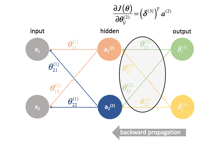
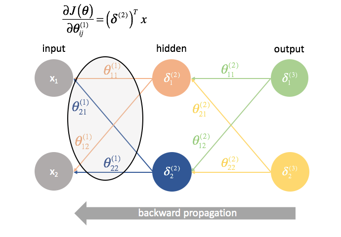
$$ \frac{{\partial J\left( \theta \right)}}{{\partial \theta _{ij}^{(l)}}} = {\left( {{\delta ^{(l + 1)}}} \right)^T}{a^{(l)}} $$

Backpropagation visualized

Before defining the formal method for backpropagation, I'd like to provide a visualization of the process.

First, we have to compute the output of a neural network via forward propagation.

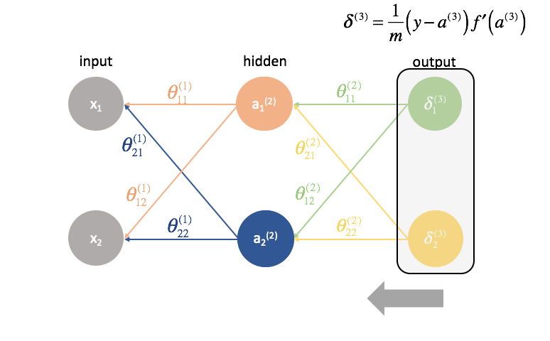
Next, we compute the ${\delta ^{(3)}}$ terms for the last layer in the network. Remember, these $\delta$ terms consist of all of the partial derivatives that will be used again in calculating parameters for layers further back. In practice, we typically refer to $\delta$ as the "error" term.

${\Theta ^{(2)}}$ is the matrix of parameters that connects layer 2 to 3. We multiply the error from the third layer by the inputs in the second layer to calculate our partial derivatives for this set of parameters.

Next, we "send back" the "error" terms in the exact same manner that we "send forward" the inputs to a neural network. The only difference is that time, we're starting from the back and we're feeding an error term, layer by layer, backwards through the network. Hence the name: backpropagation. The act of "sending back our error" is accomplished via the expression ${\delta ^{(3)}}{\Theta ^{(2)}}$.

${\Theta ^{(1)}}$ is the matrix of parameters that connects layer 1 to 2. We multiply the error from the second layer by the inputs in the first layer to calculate our partial derivatives for this set of parameters.

For every layer except for the last, the "error" term is a linear combination of parameters connecting to the next layer (moving forward through the network) and the "error" terms of that next layer. This is true for all of the hidden layers, since we don't compute an "error" term for the inputs.

The last layer is a special case because we calculate the $\delta$ values by directly comparing each output neuron to its expected output.

A formalized method for implementing backpropagation

Here, I'll present a practical method for implementing backpropagation through a network of layers $l=1,2,...,L$.

1. Perform forward propagation.

2. Compute the $\delta$ term for the output layer.
   [{\delta ^{(L)}} = \frac{1}{m}\left( {y - {a^{(L)}}} \right)f'\left( {{a^{(L)}}} \right)]

3. Compute the partial derivatives of the cost function with respect to all of the parameters that feed into the output layer, ${\Theta ^{(L - 1)}}$.
   [\frac{{\partial J\left( \theta \right)}}{{\partial \theta _{ij}^{(L-1)}}} = {\left( {{\delta ^{(L)}}} \right)^T}{a^{(L-1)}}]

4. Go back one layer.
   $l = l - 1$

5. Compute the $\delta$ term for the current hidden layer.
   [{\delta ^{(l)}} = {\delta ^{(l + 1)}}{\Theta ^{(l)}}f'\left( {{a^{(l)}}} \right)]

6. Compute the partial derivatives of the cost function with respect to all of the parameters that feed into the current layer.
   [\frac{{\partial J\left( \theta \right)}}{{\partial \theta _{ij}^{(l)}}} = {\left( {{\delta ^{(l + 1)}}} \right)^T}{a^{(l)}}]

7. Repeat 4 through 6 until you reach the input layer.

Revisiting the weights initialization

When we started, I proposed that we just randomly initialize our weights in order to have a place to start. This allowed us to perform forward propagation, compare the outputs to the expected values, and compute the cost of our model.

It's actually very important that we initialize our weights to random values so that we can break the symmetry in our model. If we had initialized all of our weights to be equal to be the same, every neuron in the next layer forward would be equal to the same linear combination of values.

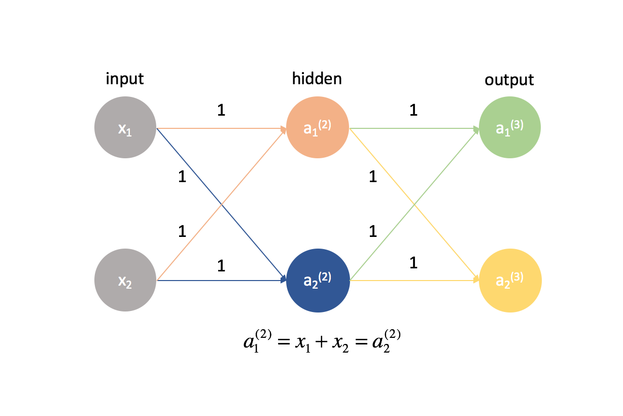
By this same logic, the $\delta$ values would also be the same for every neuron in a given layer.

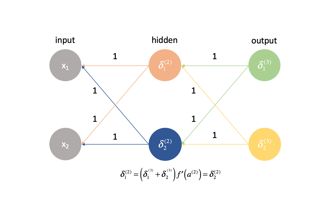
Further, because we calculate the partial derivatives in any given layer by combining $\delta$ values and activations, all of the partial derivatives in any given layer would be identical. As such, the weights would update symmetrically in gradient descent and multiple neurons in any layer would be useless. This obviously would not be a very helpful neural network.

Randomly initializing the network's weights allows us to break this symmetry and update each weight individually according to its relationship with the cost function. Typically we'll assign each parameter to a random value in $\left[ { - \varepsilon ,\varepsilon } \right]$ where $\varepsilon$ is some value close to zero.

Putting it all together

After we've calculated all of the partial derivatives for the neural network parameters, we can use gradient descent to update the weights.

In general, we defined gradient descent as
[{\theta _i}: = {\theta _i} + \Delta {\theta _i}]

where $\Delta {\theta _i}$ is the "step" we take walking along the gradient, scaled by a learning rate, $\eta$.

[\Delta {\theta _i} = - \eta \frac{{\partial J\left( \theta \right)}}{{\partial {\theta _i}}}]

We'll use this formula to update each of the weights, recompute forward propagation with the new weights, backpropagate the error, and calculate the next weight update. This process continues until we've converged on an optimal value for our parameters.

During each iteration we perform forward propagation to compute the outputs and backward propagation to compute the errors; one complete iteration is known as an epoch. It is common to report evaluation metrics after each epoch so that we can watch the evolution of our neural network as it trains.

Further reading

• The Matrix Calculus You Need For Deep Learning

• How the backpropagation algorithm works

• Stanford cs231n: Backpropagation, Intuitions

• CS231n Winter 2016: Lecture 4: Backpropagation, Neural Networks 1

• Lectures on Deep Learning

• Yes you should understand backprop

• Building blocks of neural networks

• And in case you just gave up on backpropagation... Deep Learning without Backpropagation