
Gradient descent is an optimization technique commonly used in training machine learning algorithms. Often when we're building a machine learning model, we'll develop a cost function which is capable of measuring how well our model is doing. This function will penalize any error our model makes (by assigning a cost) with respect to the current parameter values. Thus, by minimizing the cost function we can find the optimal parameters that yield the best model performance.
Common cost functions:
- Mean squared error
- Cross-entropy loss (log loss)
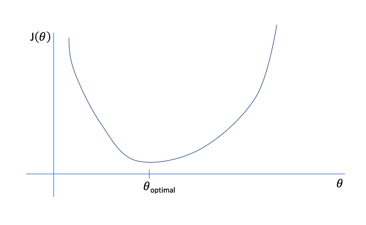
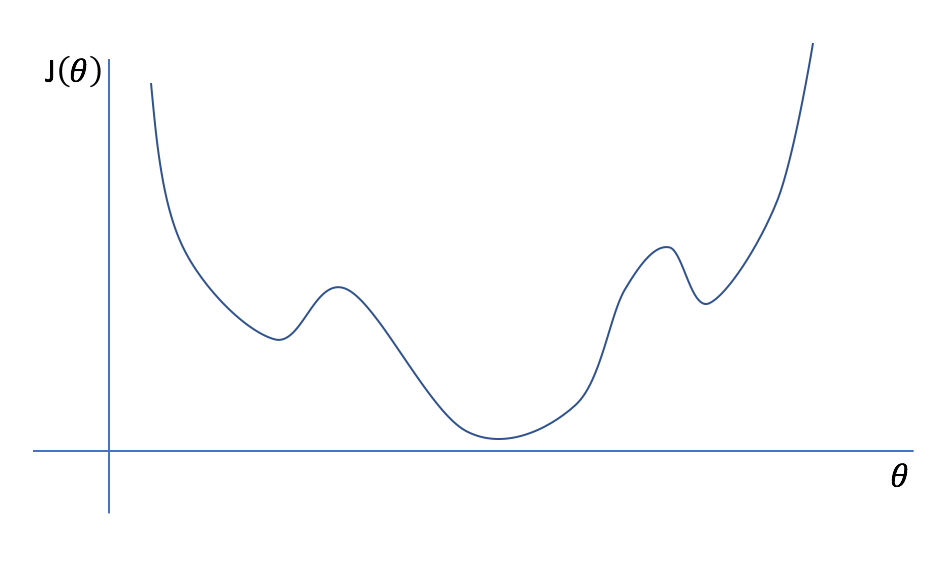
Let's start off with an extremely simple example of a model with only one parameter. We can plot an arbitrary cost function, $J\left( \theta \right)$, as a function of $\theta$. Viewing this plot, it is easy to see what the best parameter for the model is (labeled as $\theta _{optimal}$) as it leads to the least amount of error possible in the model.
However, it would be computationally expensive to calculate the cost function for every possible parameter value. Instead, let's start with an initial guess and iteratively refine it.
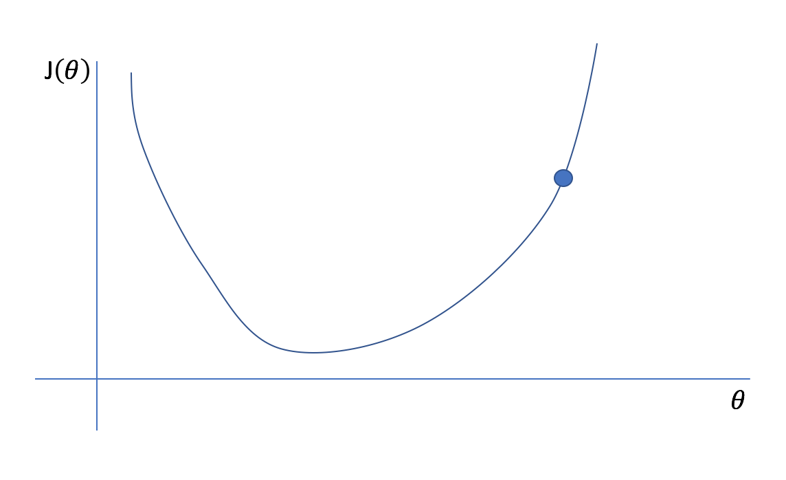
Remember, we don't actually know what the plotted cost function looks like (imagine how computationally expensive it would be for a model with 100 parameters!), we only know what the cost function is at our initial guess. Fortunately, we constructed our cost function so that it was continuous and differentiable. Thus, we also know the instantaneous slope of the cost function at our current position. For multivariate functions, we cn calculate the gradient which represents the instantaneous slope of the function with respect to each parameter. (Hence the name of our optimization technique, gradient descent.) We can find the minimum point of a function by iteratively taking steps in the opposite direction of the instantaneous slope.
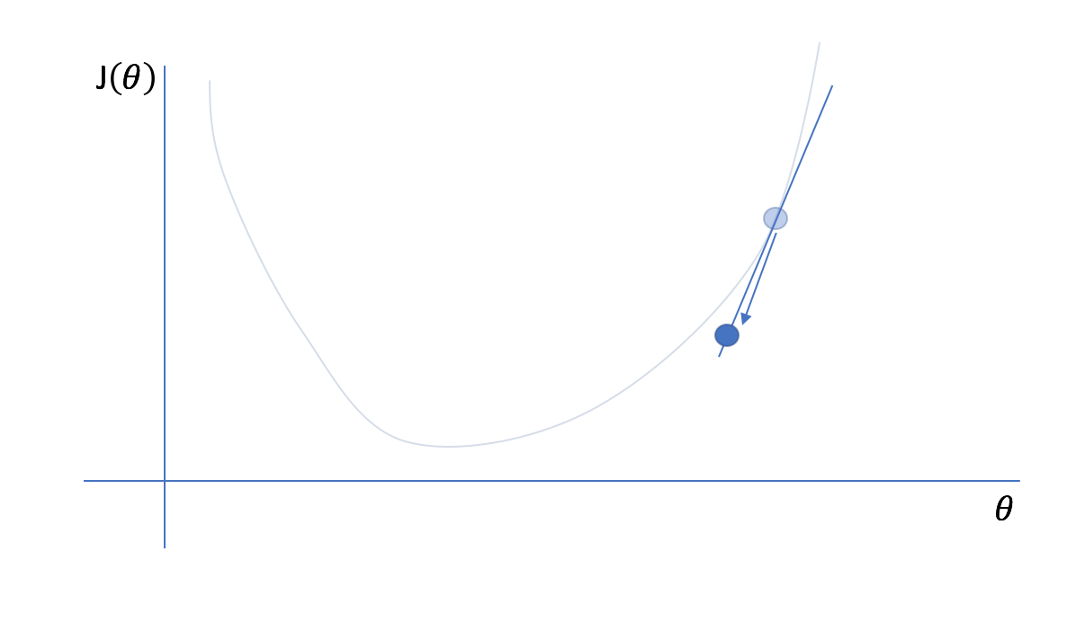
Next, we'll reevaluate the cost function and its gradient at our new parameter value...
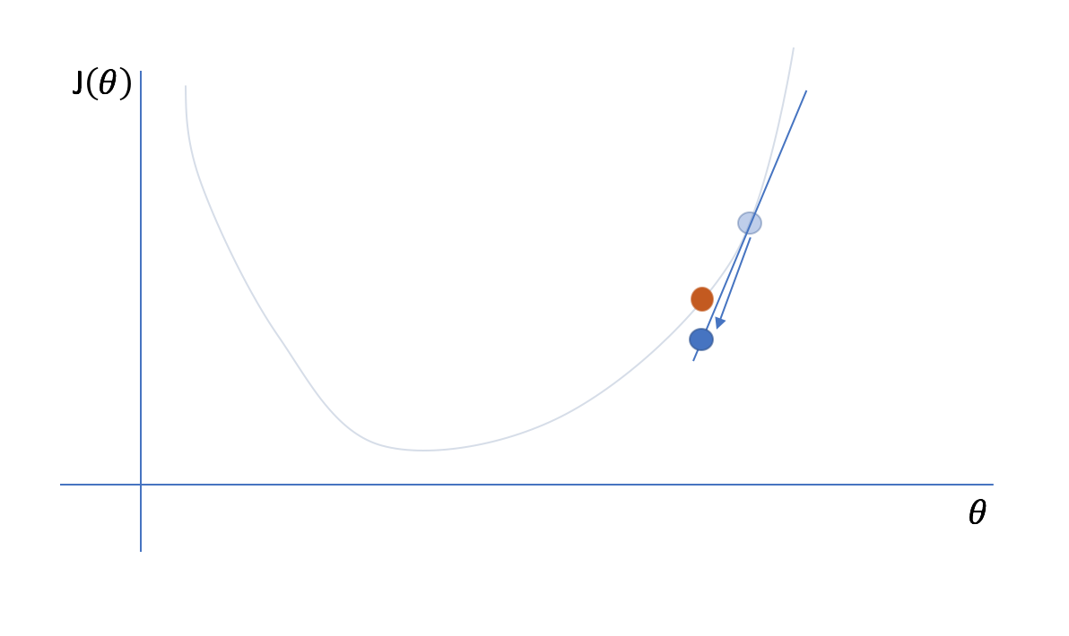
and then iteratively repeat this process of taking a step in the opposite direction of the gradient and then reevaluating the cost function and its gradient.
Generally, we can define the process of gradient descent as
[{\theta _i}: = {\theta _i} + \Delta {\theta _i}]
where
[\Delta {\theta_i} = - \alpha \frac{{\partial J\left( \theta \right)}}{{\partial {\theta_i}}}]
$\Delta {\theta_i}$ is the "step" we take walking along the gradient, and we set a learning rate, $\alpha$, to control the size of our steps.
For the case of a univariate cost function, we can only move along the cost function by moving forwards or backwards in one dimension. However, for multivariate cost functions, you can move along the cost function in any number of directions. Conveniently, the gradient of the cost function corresponds with the direction of greatest descent. Thus, we can extend our approach to a multivariate cost function as an efficient way to optimize our model's parameters.
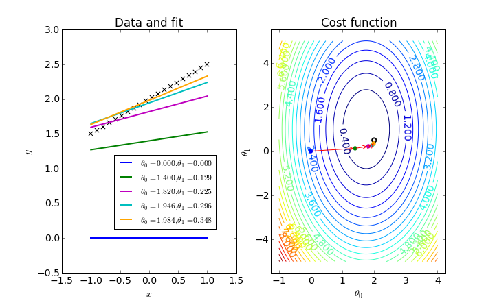
The following figure displays a gradient descent optimization of a linear regression model, where two parameters are optimized by finding the minimum value on the 3D cost function (represented by a contour plot).
Some people describe gradient descent as follows:
Say you're on the top of a mountain and you want to figure out how to get to the bottom. With gradient descent, you'll simply look around in all possible directions and take a step in the steepest downhill direction. Then you'll look around again and take another step in the steepest downhill direction. You'll continue this process until you get to the bottom.
However, gradient descent is actually quite a bit more elegant in that we don't have to look around in every direction to find the steepest downhill direction. We can find this direction in one swift calculation of the gradient!
As you reach a local optima, the slope will approach zero. Once the slope of your current parameter reaches zero, your parameter value will stop updating. While this is generally useful as it results in convergence and signifies that we can stop the iterative process, it can pose a problem when the gradient descent finds a local optimum (see example in the figure below). To prevent gradient descent from getting stuck at local optima (which may not be the global optimum), we can use a momentum term which allows our search to overcome local optima. Further, in some cases we can develop cost functions which are proven to have a convex space, guaranteeing that we only have one optimum, the global minimum.
Mini batch gradient descent
In general, when computing the cost function we look at the loss associated with each training example and then sum these values together for an overall cost of the entire dataset. This is the most basic form of gradient descent, also known as batch gradient descent since we compute the cost in one large batch computation.
However, for big datasets this can take a long time to compute. Moreover, it begs the question: do we really need to see all of the data before making improvements to our parameter values?
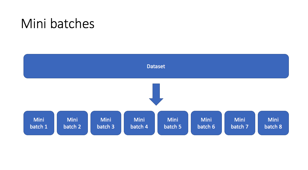
Mini batch gradient descent allows us to split our training data into mini batches which can be processed individually. When each mini batch is processed, we look at the cost function relative to the data from the current mini batch and update our parameters accordingly. Then we continue to do this iterating over all of the mini batches until we've seen the whole dataset. One full cycle through the dataset is referred to as an epoch.
This allows us to improve our model parameters at each mini batch iteration. If we split our data into 100 mini batches, this would allow us to take 100 steps towards the global optimum rather than just 1 step had we elected to use batch gradient descent. This said, because we're updating our parameters on a more narrow view of the data, we introduce a degree of variance into our optimization process. Although we will generally still follow the direction towards the global minimum, we're no longer guarunteed that each step will bring us closer to the optimal parameter values.
At the extreme case, we can set a mini batch size equal to one where we perform an update on a single training observation. This is known as stochastic gradient descent. On the other extreme, a batch size equal to the number of training examples would represent batch gradient descent. Mini batch gradient descent lies somewhere in the middle of that spectrum, with common batch sizes including: 64, 128, 256, and 512. Finding the optimal batch size will yield the fastest learning.
Advanced techniques
Now that you have a basic understanding for the gradient descent process, we can discuss more advanced optimization algorithms that promise faster learning than standard gradient descent.
Ultimately, the following techniques are adaptations to the standard gradient descent equation in hopes of improving convergence properties. I introduced the concept of gradient descent with an example finding the optimal value (lowest cost) for a single parameter. However, some machine learning models contain millions of parameters, meaning we're optimizing a cost function over millions of dimensions.
These cost functions can be quite complex. Ideally, we want to find the global minimum of the function, which represents the best possible parameter values to optimize our selected evaluation metric, given the design of our model. Depending on where we start, we'll encounter local minimum and saddlepoints along the way. Fortunately, because we're dealing with such a high dimensional space, the odds of having a minimum value in all dimensions is quite low, so saddle points are much more common.
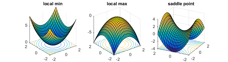
Photo by Rong Ge
Unforunately, saddle points can slow down or halt the optimization process as shown in the examples below. As you can see, the stochastic gradient descent prematurely converges to a suboptimal value. The other points are all variations of the standard gradient descent that allow for faster training with improved convergence.
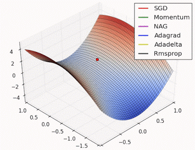
Photo by Alec Radford
Recall that for gradient descent we're taking a step along the gradient in each dimension. Notice how in the first animation we get stuck oscillating around the local minimum of one dimension and aren't able to continue downward because we're at the local maximum of the other dimension (and thus the gradient is close to zero). Because our step size in a given dimension is determined by the gradient value, we're slowed down in the presence of local optima.
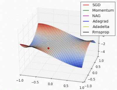
Photo by Alec Radford
Momentum
One approach to this problem is to use a moving average gradient instead of the immediate gradient at each time step. By using an average gradient over the previous $x$ steps, we're able to keep momentum when we approach local optima. As you approach the optima your immediate gradient will get smaller, but because you're averaging over $x$ timesteps, we're don't slow down as drastically as we would if we only used the immediate gradient value.
This said, it's still possible to get stuck at a saddle point if we only have momentum in the direction of the minimum. You can see this in the first animation, where the momentum optimizer fails to exit the local optima.
In order to implement momentum, we'll keep track (incrementally) of the moving average gradient, where $\beta$ is a hyperparameter of the optimization scheme. $\beta$ essentially controls how far back we'll look when calculating our moving average. For example, a common value for $\beta$ is 0.9 which tracks the moving average of the last 10 timesteps.
[{v_{dW}} = \beta {v_{dW}} + \left( {1 - \beta } \right)dW]
[{v_{db}} = \beta {v_{db}} + \left( {1 - \beta } \right)db]
Note: Some formulas for moving average will have a bias correction, but this implementation typically disregards it.
This is sometimes referred to as the velocity term.
Next, when updating the gradients, we'll use the velocity term in place of the immediate gradient value.
[W = W - \alpha {v_{dW}}]
[b = b - \alpha {v_{db}}]
Momentum offers improvements navigating ravines, reducing back and forth oscillations (because in a moving average those would cancel out) and focusing on the steepest descent path.
RMSProp
As mentioned previously, momentum can still have its shortfalls. Geoff Hinton introduced an alternative optimization scheme, RMSProp, in a Coursera course. This technique aims to prevent local optima from slowing our convergence process by adaptively scaling the learning rate in each dimension according to the exponentially weight average of the gradient.
We keep track of the exponentially weighted average of the gradient in each dimension using the following equation, where $\beta$ again represents a hyperparameter that controls how far back we look when computing the exponential moving average.
[{s_{dW}} = \beta {s_{dW}} + \left( {1 - \beta } \right)d{W^2}]
[{s_{db}} = \beta {s_{db}} + \left( {1 - \beta } \right)d{b^2}]
We can then update our paramters using the standard form of gradient descent, but scale the learning rate $\alpha$ by our exponentially weighted average.
[W = W - \frac{\alpha }{{\sqrt {{s_{dW}}} }}dW]
[b = b - \frac{\alpha }{{\sqrt {{s_{db}}} }}db]
This has the effect of dampening out steep gradients as to reduce oscillations within ravines during our journey to the global optimum.
Adam
Adam, which stands for Adaptive Moment Estimation, combines the two previous ideas of using a moving average gradient (momentum) and adaptive learning rates (RMSProp). These two values respectively represent the estimates of the first and second moment of the gradients, hence the name of the technique.
We'll calculate the first and second moments, $v$ and $s$, using two separate $\beta$ values.
[{v_{dW}} = {\beta_1}{v_{dW}} + \left( {1 - {\beta_1}} \right)dW]
[{s_{dW}} = {\beta_2}{s_{dW}} + \left( {1 - {\beta_2}} \right)d{W^2}]
[{v_{db}} = {\beta_1}{v_{db}} + \left( {1 - {\beta_1}} \right)db]
[{s_{db}} = {\beta_2}{s_{db}} + \left( {1 - {\beta_2}} \right)d{b^2}]
For this technique, we do apply bias correction to the moving averages.
[v_{dW}^{corrected} = \frac{{{v_{dW}}}}{{1 - \beta_1^t}}]
[v_{db}^{corrected} = \frac{{{v_{db}}}}{{1 - \beta_1^t}}]
[s_{dW}^{corrected} = \frac{{{s_{dW}}}}{{1 - \beta_2^t}}]
[s_{db}^{corrected} = \frac{{{s_{db}}}}{{1 - \beta_2^t}}]
We can then update our parameter values as follows.
[W = W - \frac{\alpha }{{\sqrt {s_{dW}^{corrected}} + \varepsilon }}v_{dW}^{corrected}]
[b = b - \frac{\alpha }{{\sqrt {s_{db}^{corrected}} + \varepsilon }}v_{db}^{corrected}]
Note: This update rule will have an added $\epsilon$ in the denominator to prevent divide by zero errors. A typical value for $\epsilon$ is $10^8$.
For this optimization scheme, we'll typically use $\beta_1=0.9$, and $\beta_2 =0.999$ as the initial hyperparamter values.
Further reading
- Setting the learning rate of your neural network
- An overview of gradient descent optimization algorithms: Sebastian Ruder
- Optimization: Stochastic Gradient Descent
- The Marginal Value of Adaptive Gradient Methods in Machine Learning
- More advanced gradient descent techniques
- An Interactive Tutorial on Numerical Optimization
- Learning: tips for neural networks
- Intro to optimization in deep learning: Momentum, RMSProp and Adam