Setting the learning rate of your neural network.
In previous posts, I've discussed how we can train neural networks using backpropagation with gradient descent. One of the key hyperparameters to set in order to train a neural network is the learning rate for gradient descent.

In previous posts, I've discussed how we can train neural networks using backpropagation with gradient descent. One of the key hyperparameters to set in order to train a neural network is the learning rate for gradient descent. As a reminder, this parameter scales the magnitude of our weight updates in order to minimize the network's loss function.
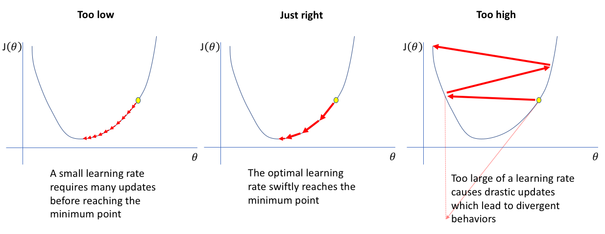
If your learning rate is set too low, training will progress very slowly as you are making very tiny updates to the weights in your network. However, if your learning rate is set too high, it can cause undesirable divergent behavior in your loss function. I'll visualize these cases below - if you find these visuals hard to interpret, I'd recommend reading (at least) the first section in my post on gradient descent.
So how do we find the optimal learning rate?
3e-4 is the best learning rate for Adam, hands down.
— Andrej Karpathy (@karpathy) November 24, 2016
Perfect! I guess my job here is done.
Well... not quite.
(i just wanted to make sure that people understand that this is a joke...)
— Andrej Karpathy (@karpathy) November 24, 2016
(Humor yourself by reading through that thread after finishing this post.)
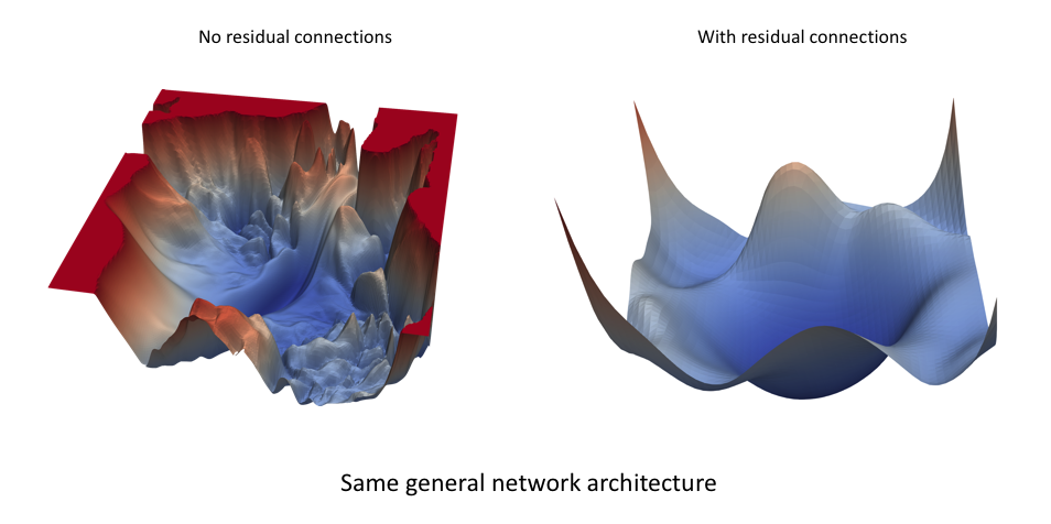
The loss landscape of a neural network (visualized below) is a function of the network's parameter values quantifying the "error" associated with using a specific configuration of parameter values when performing inference (prediction) on a given dataset. This loss landscape can look quite different, even for very similar network architectures. The images below are from a paper, Visualizing the Loss Landscape of Neural Nets, which shows how residual connections in a network can yield an smoother loss topology.
The optimal learning rate will be dependent on the topology of your loss landscape, which is in turn dependent on both your model architecture and your dataset. While using a default learning rate (ie. the defaults set by your deep learning library) may provide decent results, you can often improve the performance or speed up training by searching for an optimal learning rate. I hope you'll see in the next section that this is quite an easy task.
A systematic approach towards finding the optimal learning rate
Ultimately, we'd like a learning rate which results is a steep decrease in the network's loss. We can observe this by performing a simple experiment where we gradually increase the learning rate after each mini batch, recording the loss at each increment. This gradual increase can be on either a linear or exponential scale.
For learning rates which are too low, the loss may decrease, but at a very shallow rate. When entering the optimal learning rate zone, you'll observe a quick drop in the loss function. Increasing the learning rate further will cause an increase in the loss as the parameter updates cause the loss to "bounce around" and even diverge from the minima. Remember, the best learning rate is associated with the steepest drop in loss, so we're mainly interested in analyzing the slope of the plot.
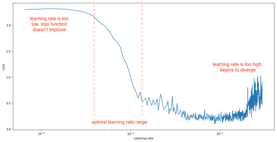
You should set the range of your learning rate bounds for this experiment such that you observe all three phases, making the optimal range trivial to identify.
This technique was proposed by Leslie Smith in Cyclical Learning Rates for Training Neural Networks and evangelized by Jeremy Howard in fast.ai's course.
Setting a schedule to adjust your learning rate during training
Another commonly employed technique, known as learning rate annealing, recommends starting with a relatively high learning rate and then gradually lowering the learning rate during training. The intuition behind this approach is that we'd like to traverse quickly from the initial parameters to a range of "good" parameter values but then we'd like a learning rate small enough that we can explore the "deeper, but narrower parts of the loss function" (from Karparthy's CS231n notes). If you're having a hard time picturing what I just mentioned, recall that too high of a learning rate can cause the parameter update to "jump over" the ideal minima and subsequent updates will either result in a continued noisy convergence in the general region of the minima, or in more extreme cases may result in divergence from the minima.
The most popular form of learning rate annealing is a step decay where the learning rate is reduced by some percentage after a set number of training epochs.
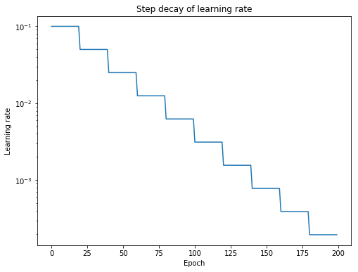
More generally, we can establish that it is useful to define a learning rate schedule in which the learning rate is updating during training according to some specified rule.
Cyclical learning rates
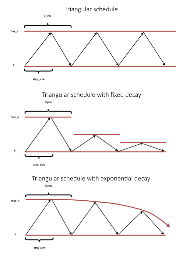
In the previously mentioned paper, Cyclical Learning Rates for Training Neural Networks, Leslie Smith proposes a cyclical learning rate schedule which varies between two bound values. The main learning rate schedule (visualized below) is a triangular update rule, but he also mentions the use of a triangular update in conjunction with a fixed cyclic decay or an exponential cyclic decay.
Note: At the end of this post, I'll provide the code to implement this learning rate schedule. Thus, if you don't care to understand the mathematical formulation you can skim past this section.
We can write the general schedule as
$$ {\eta_t} = {\eta_{\min }} + \left( {{\eta_{\max }} - {\eta_{\min }}} \right)\left( {\max \left( {0,1 - x} \right)} \right) $$
where $x$ is defined as
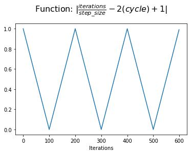
$$ x = \left| {\frac{{iterations}}{stepsize} - 2\left( {cycle} \right) + 1} \right| $$
and $cycle$ can be calculated as
$$ cycle = floor\left( 1 + {\frac{{iterations}}{{2\left( {stepsize} \right)}}} \right) $$
where $\eta_{\min }$ and $\eta_{\max }$ define the bounds of our learning rate, $iterations$ represents the number of completed mini-batches, $stepsize$ defines one half of a cycle length. As far as I can gather, $1-x$ should always be positive, so it seems the $\max$ operation is not strictly necessary.
In order to grok how this equation works, let's progressively build it with visualizations. For the visuals below, the triangular update for 3 full cycles are shown with a step size of 100 iterations. Remember, one iteration corresponds with one mini-batch of training.
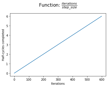
Foremost, we can establish our "progress" during training in terms of half-cycles that we've completed. We measure our progress in terms of half-cycles and not full cycles so that we can acheive symmetry within a cycle (this should become more clear as you continue reading).
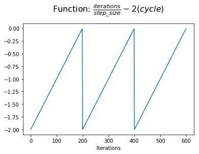
Next, we compare our half-cycle progress to the number of half-cycles which will be completed at the end of the current cycle. At the beginning of a cycle, we have two half-cycles yet to be completed. At the end of a cycle, this value reaches zero.
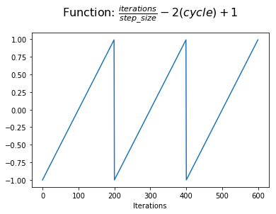
Next, we'll add 1 to this value in order to shift the function to be centered on the y-axis. Now we're showing our progress within a cycle with reference to the half-cycle point.
At this point, we can take the absolute value to acheive a triangular shape within each cycle. This is the value that we assign to $x$.
However, we'd like our learning rate schedule to start at the minumum value, increasing to the maximum value at the middle of a cycle, and then decrease back to the minimum value. We can accomplish this by simply calculating $1-x$.
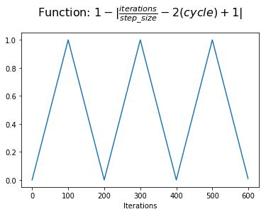
We now have a value which we can use to modulate the learning rate by adding some fraction of the learning rate range to the minimum learning rate (also referred to as the base learning rate).
Smith writes, the main assumption behind the rationale for a cyclical learning rate (as opposed to one which only decreases) is "that increasing the learning rate might have a short term negative effect and yet achieve a longer term beneficial effect." Indeed, his paper includes several examples of a loss function evolution which temporarily deviates to higher losses while ultimately converging to a lower loss when compared with a benchmark fixed learning rate.
To gain intuition on why this short-term effect would yield a long-term positive effect, it's important to understand the desirable characteristics of our converged minimum. Ultimately, we'd like our network to learn from the data in a manner which generalizes to unseen data. Further, a network with good generalization properties should be robust in the sense that small changes to the network's parameters don't cause drastic changes to performance. With this in mind, it makes sense that sharp minima lead to poor generalization as small changes to the parameter values may result in a drastically higher loss. By allowing for our learning rate to increase at times, we can "jump out" of sharp minima which would temporarily increase our loss but may ultimately lead to convergence on a more desirable minima.
Note: Although the "flat minima for good generalization" is widely accepted, you can read a good counter-argument here.
Additionally, increasing the learning rate can also allow for "more rapid traversal of saddle point plateaus." As you can see in the image below, the gradients can be very small at a saddle point. Because the parameter updates are a function of the gradient, this results in our optimization taking very small steps; it can be useful to increase the learning rate here to avoid getting stuck for too long at a saddle point.
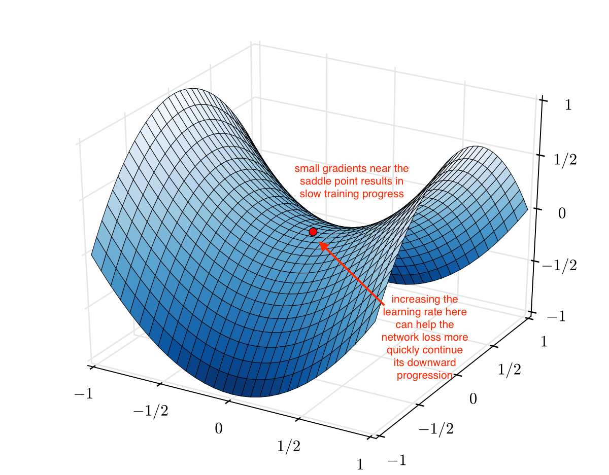
Image credit (with modification)
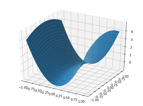
Note: A saddle point, by definition, is a critical point in which some dimensions observe a local minimum while other dimensions observe a local maximum. Because neural networks can have thousands or even millions of parameters, it's unlikely that we'll observe a true local minimum across all of these dimensions; saddle points are much more likely to occur. When I referred to "sharp minima", realistically we should picture a saddle point where the minimum dimensions are very steep while the maximum dimensions are very wide (as shown below).
Stochastic Gradient Descent with Warm Restarts (SGDR)
A similar approach cyclic approach is known as stochastic gradient descent with warm restarts where an aggressive annealing schedule is combined with periodic "restarts" to the original starting learning rate.
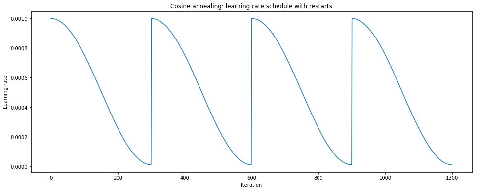
We can write this schedule as
$$ {\eta_t} = \eta_{\min }^i + \frac{1}{2}\left( {\eta_{\max }^i - \eta_{\min }^i} \right)\left( {1 + \cos \left( {\frac{{{T_{current}}}}{{{T_i}}}} \pi \right) } \right) $$
where ${\eta_t}$ is the learning rate at timestep $t$ (incremented each mini batch), ${\eta_{\max}^i}$ and ${\eta_{\min }^i}$ define the range of desired learning rates, $T_{current}$ represents the number of epochs since the last restart (this value is calculated at every iteration and thus can take on fractional values), and $T_{i}$ defines the number of epochs in an cycle. Let's try to break this equation down.
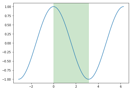
This annealing schedule relies on the cosine function, which varies between -1 and 1. ${\frac{T_{current}}{T_i}}$ is capable of taking on values between 0 and 1, which is the input of our cosine function. The corresponding region of the cosine function is highlighted below in green. By adding 1, our function varies between 0 and 2, which is then scaled by $\frac{1}{2}$ to now vary between 0 and 1. Thus, we're simply taking the minimum learning rate and adding some fraction of the specified learning rate range (${\eta_{\max }^i - \eta_{\min }^i}$). Because this function starts at 1 and decreases to 0, the result is a learning rate which starts at the maximum of the specified range and decays to the minimum value. Once we reach the end of a cycle, $T_{current}$ resets to 0 and we start back at the maximum learning rate.
The authors note that this learning rate schedule can further be adapted to:
- Lengthen the cycle as training progresses.
- Decay ${\eta_{\max }^i}$ and ${\eta_{\min }^i}$ after each cycle.
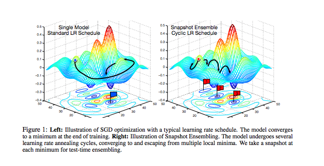
By drastically increasing the learning rate at each restart, we can essentially exit a local minima and continue exploring the loss landscape.
Neat idea: By snapshotting the weights at the end of each cycle, researchers were able to build an ensemble of models at the cost of training a single model. This is because the network "settles" on various local optima from cycle to cycle, as shown in the figure below.
Implementation
Both finding the optimal range of learning rates and assigning a learning rate schedule can be implemented quite trivially using Keras Callbacks.
Finding the optimal learning rate range
We can write a Keras Callback which tracks the loss associated with a learning rate varied linearly over a defined range.
Setting a learning rate schedule
Step Decay
For a simple step decay, we can use the LearningRateScheduler Callback.
Cyclical Learning Rate
To apply the cyclical learning rate technique, we can reference this repo which has already implemented the technique in the paper. In fact, this repo is cited in the paper's appendix.
Stochastic Gradient Descent with Restarts
Snapshot Ensembles
To apply the "Train 1, get M for free" technique, you can reference this repo.
Further reading
- Stanford CS231n: Annealing the learning rate
- Cyclical Learning Rates for Training Neural Networks
- Exploring loss function topology with cyclical learning rates
- SGDR: Stochastic Gradient Descent with Warm Restarts
- Snapshot Ensembles: Train 1, get M for free
- (extension of concept) Loss Surfaces, Mode Connectivity, and Fast Ensembling of DNNs
- (extension of concept) Loss Surfaces, Mode Connectivity, and Fast Ensembling of DNNs
- Visualizing the Loss Landscape of Neural Nets
- Optimization for Deep Learning Highlights in 2017: Sebastian Ruder
- On Large-Batch Training for Deep Learning: Generalization Gap and Sharp Minima
- Sharp Minima Can Generalize For Deep Nets
- The Two Phases of Gradient Descent in Deep Learning
- Recent Advances for a Better Understanding of Deep Learning − Part I