Learning from imbalanced data.
In this blog post, I'll discuss a number of considerations and techniques for dealing with imbalanced data when training a machine learning model. The blog post will rely heavily on a sklearn contributor package called imbalanced-learn to implement the discussed techniques.

In this blog post, I'll discuss a number of considerations and techniques for dealing with imbalanced data when training a machine learning model. The blog post will rely heavily on a sklearn contributor package called imbalanced-learn to implement the discussed techniques.
Training a machine learning model on an imbalanced dataset can introduce unique challenges to the learning problem. Imbalanced data typically refers to a classification problem where the number of observations per class is not equally distributed; often you'll have a large amount of data/observations for one class (referred to as the majority class), and much fewer observations for one or more other classes (referred to as the minority classes). For example, suppose you're building a classifier to classify a credit card transaction a fraudulent or authentic - you'll likely have 10,000 authentic transactions for every 1 fraudulent transaction, that's quite an imbalance!
To understand the challenges that a class imbalance imposes, let's consider two common ways we'll train a model: tree-based logical rules developed according to some splitting criterion, and parameterized models updated by gradient descent.
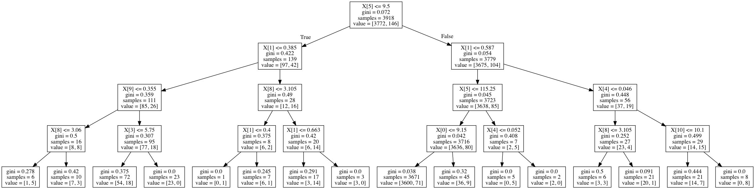
When building a tree-based model (such as a decision tree), our objective is to find logical rules which are capable of taking the full dataset and separating out the observations into their different classes. In other words, we'd like each split in the tree to increase the purity of observations such that the data is filtered into homogeneous groups. If we have a majority class present, the top of the decision tree is likely to learn splits which separate out the majority class into pure groups at the expense of learning rules which separate the minority class.
For a more concrete example, here's a decision tree trained on the wine quality dataset used as an example later on in this post. The field value represents the number of observations for each class in a given node.
Similarly, if we're updating a parameterized model by gradient descent to minimize our loss function, we'll be spending most of our updates changing the parameter values in the direction which allow for correct classification of the majority class. In other words, many machine learning models are subject to a frequency bias in which they place more emphasis on learning from data observations which occur more commonly.
It's worth noting that not all datasets are affected equally by class imbalance. Generally, for easy classification problems in which there's a clear separation in the data, class imbalance doesn't impede on the model's ability to learn effectively. However, datasets that are inherently more difficult to learn from see an amplification in the learning challenge when a class imbalance is introduced.
Metrics
When dealing with imbalanced data, standard classification metrics do not adequately represent your models performance. For example, suppose you are building a model which will look at a person's medical records and classify whether or not they are likely to have a rare disease. An accuracy of 99.5% might look great until you realize that it is correctly classifying the 99.5% of healthy people as "disease-free" and incorrectly classifying the 0.5% of people which do have the disease as healthy. I discussed this in my post on evaluating a machine learning model, but I'll provide a discussion here as well regarding useful metrics when dealing with imbalanced data.
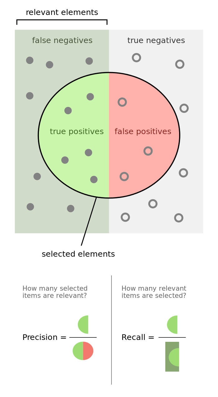
Precision is defined as the fraction of relevant examples (true positives) among all of the examples which were predicted to belong in a certain class.
$${\rm{precision}} = \frac{{{\rm{true \hspace{2mm} positives}}}}{{{\rm{true \hspace{2mm} positives + false \hspace{2mm} positives}}}}$$
Recall is defined as the fraction of examples which were predicted to belong to a class with respect to all of the examples that truly belong in the class.
$${\rm{recall}} = {\rm{ }}\frac{{{\rm{true \hspace{2mm} positives}}}}{{{\rm{true \hspace{2mm} positives + false \hspace{2mm} negatives}}}}$$
The following graphic does a phenomenal job visualizing the difference between precision and recall.
We can further combine these two metrics into a single value by calcuating the f-score as defined below.
$${F _\beta } = \left( {1 + {\beta ^2}} \right)\frac{{{\rm{precision}} \cdot {\rm{recall}}}}{{\left( {{\beta ^2} \cdot {\rm{precision}}} \right) + {\rm{recall}}}}$$
The $\beta$ parameter allows us to control the tradeoff of importance between precision and recall. $\beta < 1$ focuses more on precision while $\beta > 1$ focuses more on recall.
Another common tool used to understand a model's performance is a Receiver Operating Characteristics (ROC) curve. An ROC curve visualizes an algorithm's ability to discriminate the positive class from the rest of the data. We'll do this by plotting the True Positive Rate against the False Positive Rate for varying prediction thresholds.
$${\rm{TPR}} = {\rm{ }}\frac{{{\rm{true \hspace{2mm} positives}}}}{{{\rm{true \hspace{2mm} positives + false \hspace{2mm} negatives}}}}$$
$${\rm{FPR}} = {\rm{ }}\frac{{{\rm{false \hspace{2mm} positives}}}}{{{\rm{false \hspace{2mm} positives + true \hspace{2mm} negatives}}}}$$
For classifiers which only produce factor outcomes (ie. directly output a class), there exists a fixed TPR and FPR for a trained model. However, other classifiers, such as logistic regression, are capable of giving a probabilistic output (ie. the chance that a given observation belongs to the positive class). For these classifiers, we can specify the probability threshold by which above that amount we'll predict the observation belongs to the positive class.
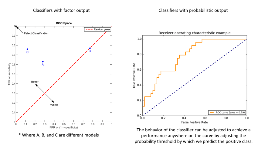
If we set a very low value for this probability threshold, we can increase our True Positive Rate as we'll be more likely to capture all of the positive observations. However, this can also introduce a number of false positive classifications, increasing our False Positive Rate. Intuitively, there exists a tradeoff between maximizing our True Positive Rate and minimizing our False Positive Rate. The ideal model would correctly identify all positive observations as belonging to the positive class (TPR=1) and would not incorrectly classify negative observations as belonging to the positive class (FPR=0).
This tradeoff can be visualized in this demonstration in which you can adjust the class distributions and classification threshold.
The area under the curve (AUC) is a single-value metric for which attempts to summarize an ROC curve to evaluate the quality of a classifier. As the name implies, this metric approximates the area under the ROC curve for a given classifier. Recall that the ideal curve hugs the upper lefthand corner as closely as possible, giving us the ability to identify all true positives while avoiding false positives; this ideal model would have an AUC of 1. On the flipside, if your model was no better than a random guess, your TPR and FPR would increase in parallel to one another, corresponding with an AUC of 0.5.
import matplotlib.pyplot as plt
from sklearn.metrics import roc_curve, roc_auc_score

preds = model.predict(X_test)
fpr, tpr, thresholds = roc_curve(y_test, preds, pos_label=1)

auc = roc_auc_score(y_test, preds)

fig, ax = plt.subplots()
ax.plot(fpr, tpr)
ax.plot([0, 1], [0, 1], color='navy', linestyle='--', label='random')
plt.title(f'AUC: {auc}')
ax.set_xlabel('False positive rate')
ax.set_ylabel('True positive rate')
Class weight
One of the simplest ways to address the class imbalance is to simply provide a weight for each class which places more emphasis on the minority classes such that the end result is a classifier which can learn equally from all classes.
To calculate the proper weights for each class, you can use the sklearn utility function shown in the example below.
from sklearn.utils.class_weight import compute_class_weight
weights = compute_class_weight('balanced', classes, y)
In a tree-based model where you're determining the optimal split according to some measure such as decreased entropy, you can simply scale the entropy component of each class by the corresponding weight such that you place more emphasis on the minority classes. As a reminder, the entropy of a node can be calculated as
$$ \mathop - \sum \limits_i^{} {p_i}{\log}\left( {{p_i}} \right) $$
where $p_i$ is the fraction of data points within class $i$.
In a gradient-based model, you can scale the calculated loss for each observation by the appropriate class weight such that you place more significance on the losses associated with minority classes. As a reminder, a common loss function for classification is the categorical cross entropy (which is very similar to the above equation, albeit with slight differences). This may be calculated as
$$ -\sum_i y_i \log \hat{y}_ i $$
where $y_i$ represents the true class (typically a one-hot encoded vector) and $\hat{y}_ i$ represents the predicted class distribution.
Oversampling
Another approach towards dealing with a class imbalance is to simply alter the dataset to remove such an imbalance. In this section, I'll discuss common techniques for oversampling the minority classes to increase the number of minority observations until we've reached a balanced dataset.
Random oversampling
The most naive method of oversampling is to randomly sample the minority classes and simply duplicate the sampled observations. With this technique, it's important to note that you're artificially reducing the variance of the dataset.
SMOTE
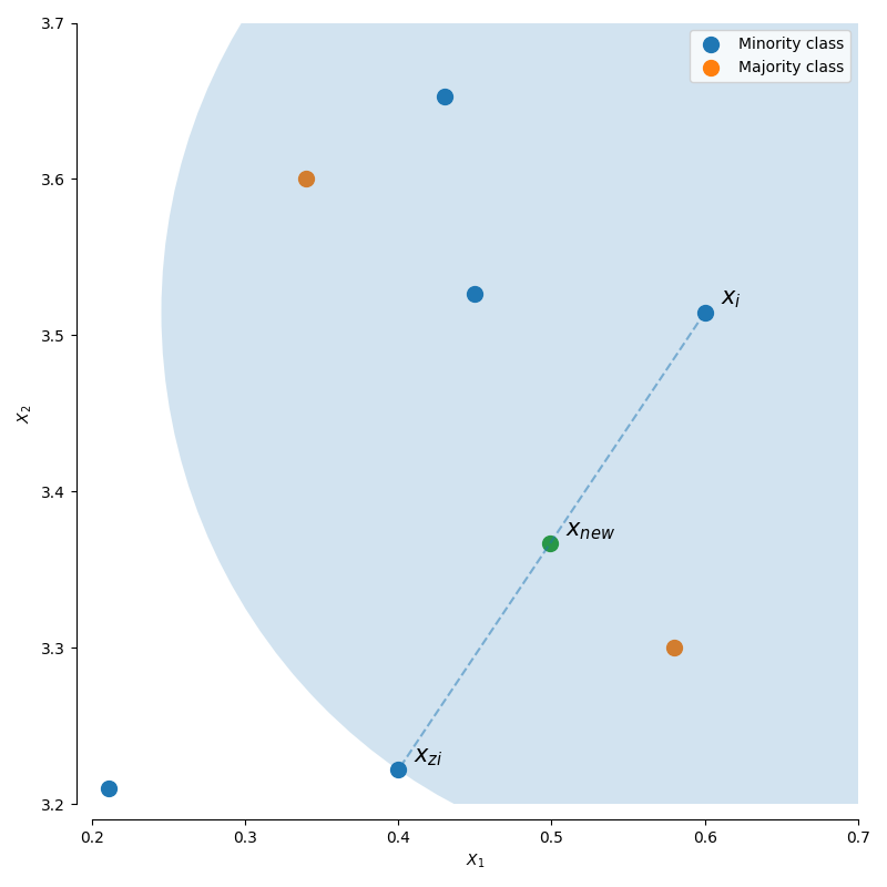
However, we can also use our existing dataset to synthetically generate new data points for the minority classes. Synthetic Minority Over-sampling Technique (SMOTE) is a technique that generates new observations by interpolating between observations in the original dataset.
For a given observation $x_i$, a new (synthetic) observation is generated by interpolating between one of the k-nearest neighbors, $x_{zi}$.
$$x_{new} = x_i + \lambda (x_{zi} - x_i)$$
where $\lambda$ is a random number in the range $\left[ {0,1} \right]$. This interpolation will create a sample on the line between $x_{i}$ and $x_{zi}$.
This algorithm has three options for selecting which observations, $x_i$, to use in generating new data points.
regular: No selection rules, randomly sample all possible $x_i$.borderline: Separates all possible $x_i$ into three classes using the k nearest neighbors of each point.- noise: all nearest-neighbors are from a different class than $x_i$
- in danger: at least half of the nearest neighbors are of the same class as $x_i$
- safe: all nearest neighbors are from the same class as $x_i$
svm: Uses an SVM classifier to identify the support vectors (samples close to the decision boundary) and samples $x_i$ from these points.
ADASYN
Adaptive Synthetic (ADASYN) sampling works in a similar manner as SMOTE, however, the number of samples generated for a given $x_i$ is proportional to the number of nearby samples which do not belong to the same class as $x_i$. Thus, ADASYN tends to focus solely on outliers when generating new synthetic training examples.
Undersampling
Rather than oversampling the minority classes, it's also possible to achieve class balance by undersampling the majority class - essentially throwing away data to make it easier to learn characteristics about the minority classes.
Random undersampling
As with oversampling, a naive implementation would be to simply sample the majority class at random until reaching a similar number of observations as the minority classes. For example, if your majority class has 1,000 observations and you have a minority class with 20 observations, you would collect your training data for the majority class by randomly sampling 20 observations from the original 1,000. As you might expect, this could potentially result in removing key characteristics of the majority class.
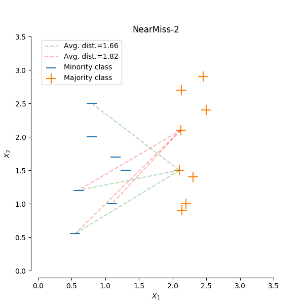
Near miss
The general idea behind near miss is to only the sample the points from the majority class necessary to distinguish between other classes.
NearMiss-1 select samples from the majority class for which the average distance of the N closest samples of a minority class is smallest.
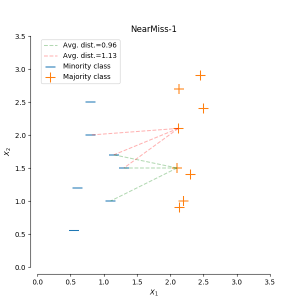
NearMiss-2 select samples from the majority class for which the average distance of the N farthest samples of a minority class is smallest.
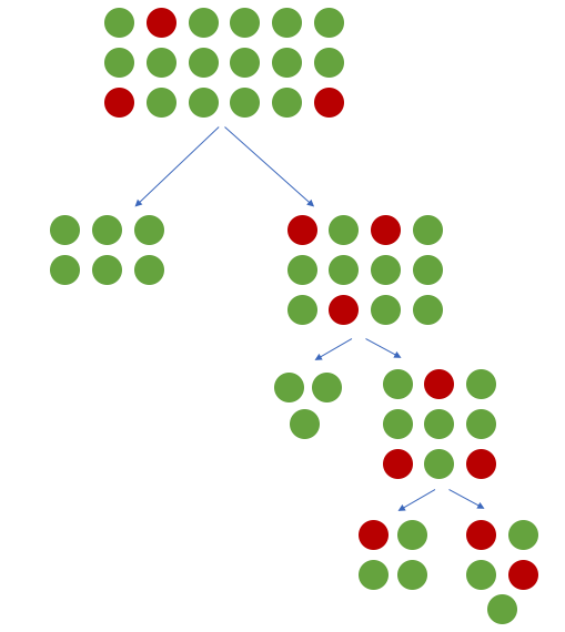
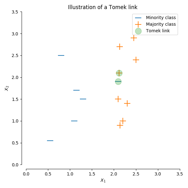
Tomeks links
A Tomek’s link is defined as two observations of different classes ($x$ and $y$) such that there is no example $z$ for which:
$$d(x, z) < d(x, y) \text{ or } d(y, z) < d(x, y)$$
where $d()$ is the distance between the two samples. In other words, a Tomek’s link exists if two observations of different classes are the nearest neighbors of each other. In the figure below, a Tomek’s link is illustrated by highlighting the samples of interest in green.
For this undersampling strategy, we'll remove any observations from the majority class for which a Tomek's link is identified. Depending on the dataset, this technique won't actually achieve a balance among the classes - it will simply "clean" the dataset by removing some noisy observations, which may result in an easier classification problem. As I discussed earlier, most classifiers will still perform adequately for imbalanced datasets as long as there's a clear separation between the classifiers. Thus, by focusing on removing noisy examples of the majority class, we can improve the performance of our classifier even if we don't necessarily balance the classes.
Edited nearest neighbors
EditedNearestNeighbours applies a nearest-neighbors algorithm and “edit” the dataset by removing samples which do not agree “enough” with their neighboorhood. For each sample in the class to be under-sampled, the nearest-neighbours are computed and if the selection criterion is not fulfilled, the sample is removed.
This is a similar approach as Tomek's links in the respect that we're not necessarily focused on actually achieving a class balance, we're simply looking to remove noisy observations in an attempt to make for an easier classification problem.
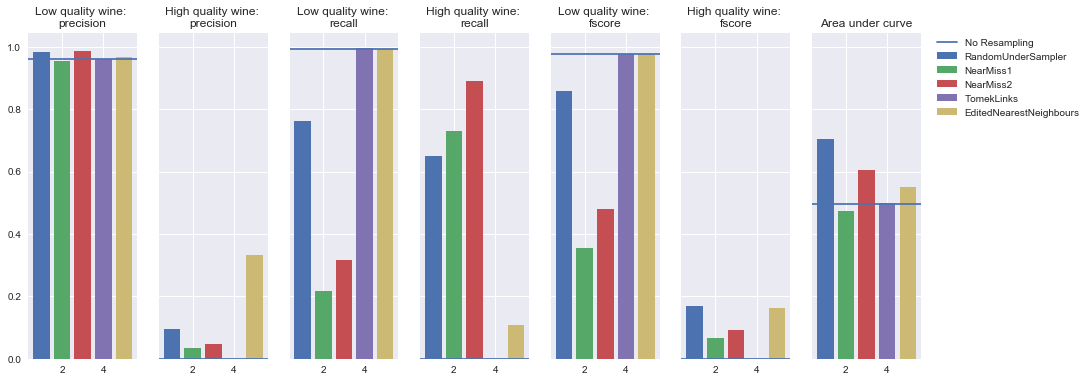
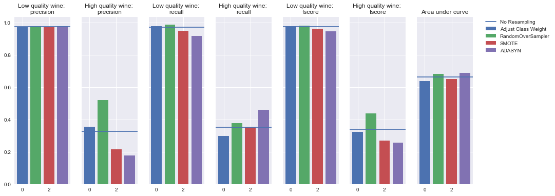
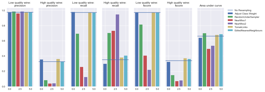
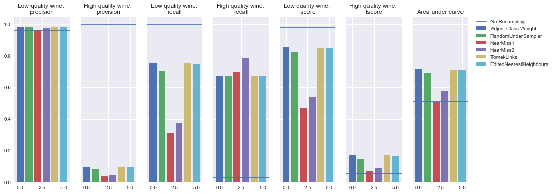
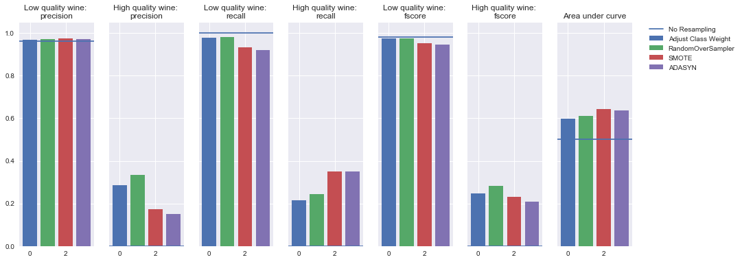
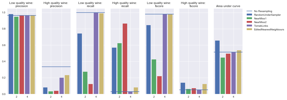
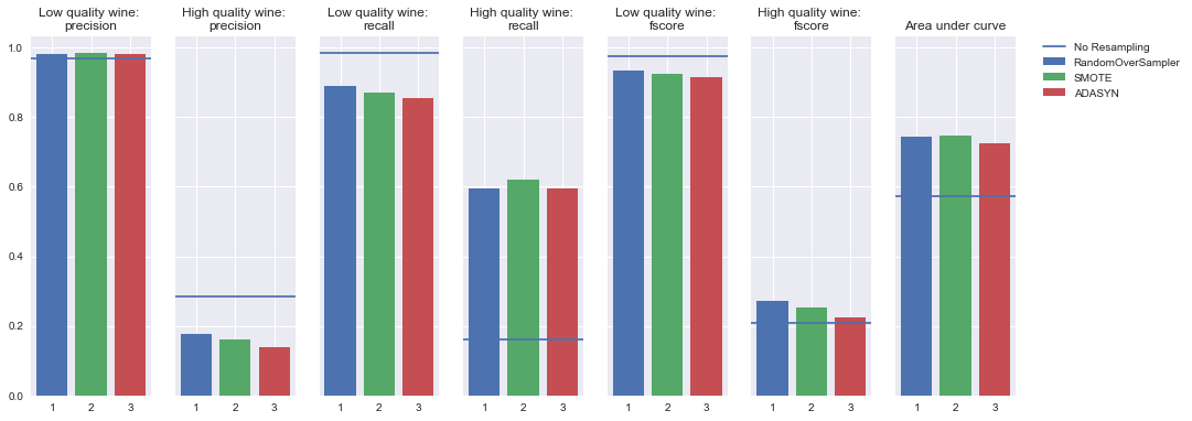
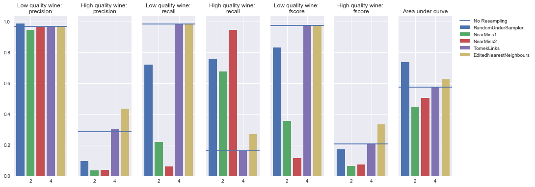
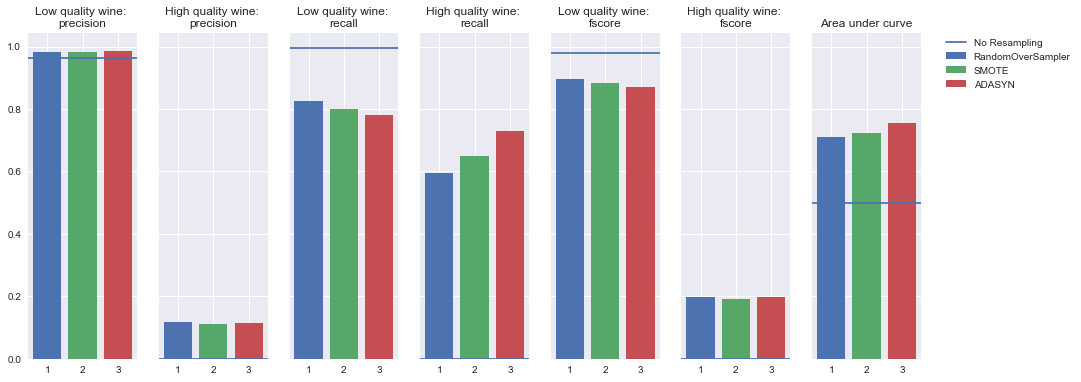
Example
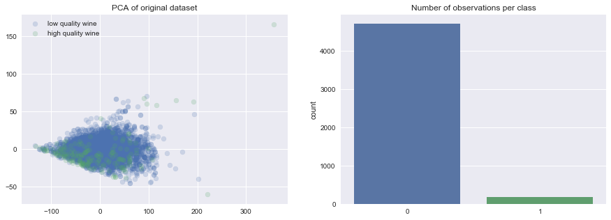
To demonstrate these various techniques, I've trained a number of models on the UCI Wine Quality dataset where I've generated my target by asserting that observations with a quality rating less than or equal to 4 are "low quality" wine and observations with a quality rating greater than or equal to 5 are "high quality" wine.
As you can see, this has introduced an imbalance between the two classes.
I'll provide the notebook I wrote to explore these techniques in a Github repo if you're interested in exploring this further. I highly encourage you to check out this notebook and perform the same experiment on a different dataset to see how it compares - let me know in the comment section!
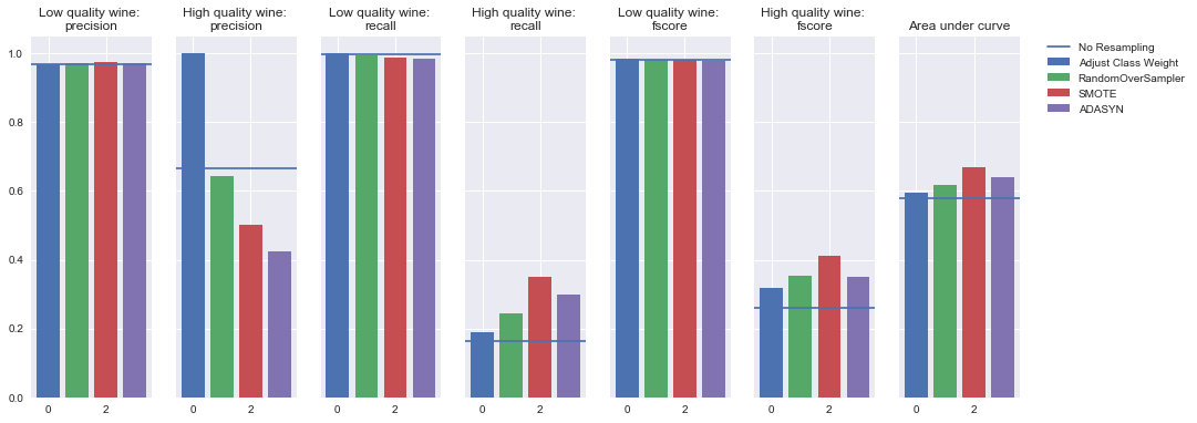
Decision tree
Oversampling
Undersampling
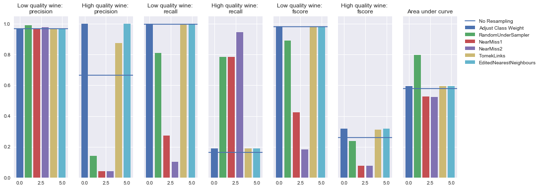
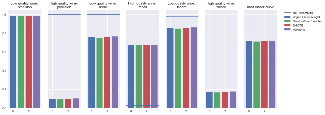
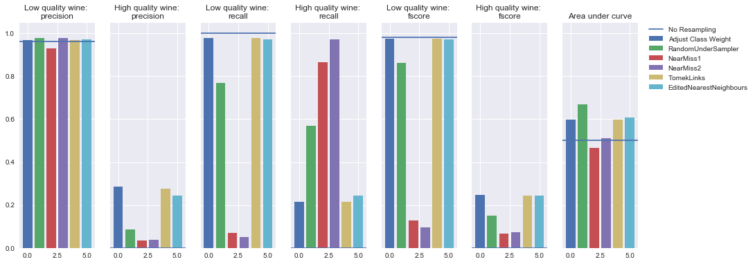
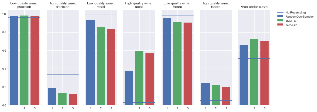
Random forest
Oversampling
Undersampling
Logistic regression
Oversampling
Undersampling
SVM Classifier
Oversampling
Undersampling
KNN
Oversampling
Undersampling
AdaBoost Classifier
Oversampling
Undersampling
Simple neural network
Oversampling
Undersampling