Understanding the Transformer architecture for neural networks
The attention mechanism allows us to merge a variable-length sequence of vectors into a fixed-size context vector. What if we could use this mechanism to entirely replace recurrence for sequential modeling? This blog post covers the Transformer architecture which explores such an approach.

In a previous post, we discussed a key innovation in sequence to sequence neural network architectures: the attention mechanism. This innovation significantly improved performance for encoder-decoder style recurrent neural network architectures by removing a bottleneck passing information from the encoder network to the decoder network. As a quick recap, before the introduction of attention we would typically summarize the entire input sequence in a single fixed-size vector to pass along as context to the decoder network. The attention mechanism allows us to merge a variable-length sequence of vectors into a fixed-size context vector at each time step in the decoder network. This provides significantly more information bandwidth to the decoder via a learnable mechanism which is capable of determining which time-steps in the input sequence are relevant at each time-step being generated in the output sequence.
Let's stop and think about that at a high-level. We have a mechanism which allows us to take a variable-length sequence and merge this information together to output a fixed-size vector. Doesn't that sound a lot like to role of a recurrent neural network? We introduced recurrence as a way to learn from variable-length sequences; but in an effort to squeeze more performance out of those recurrent networks, we accidentally stumbled across another way to process variable-length sequences.
This begs the question, what if we tried to get rid of the recurrent layers and simply used attention everywhere? This is the premise behind a seminal paper from 2017, Attention Is All You Need, which introduced the Transformer architecture for neural networks. Let's dive in and explore that idea in this blog post.
Overview
- Swapping out recurrent layers with attention
- Generalizing the attention mechanism
- Defining the Transformer architecture
- Benefits of an attention-only architecture
- Resources
Swapping out recurrent layers with attention
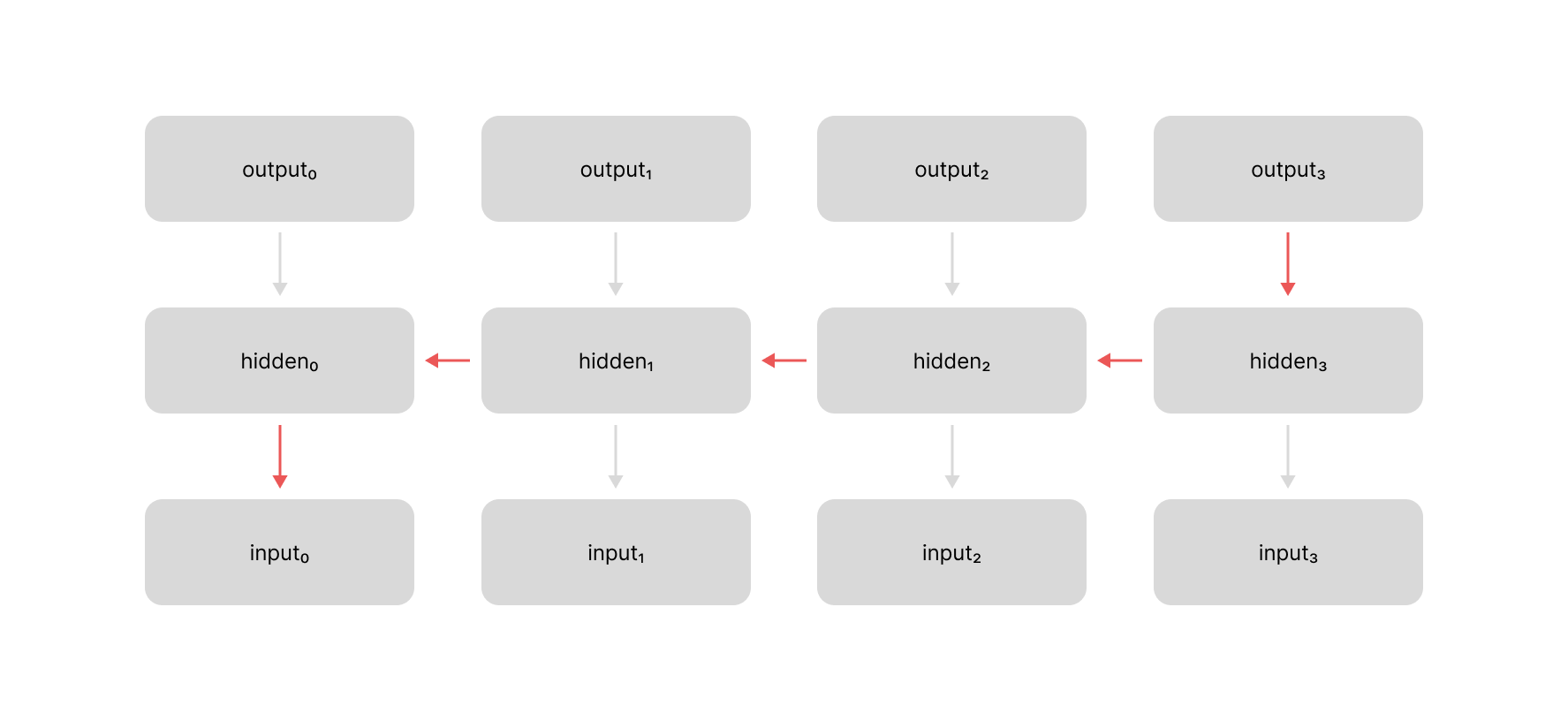
Let's first walk through what exactly it means to "replace the recurrent layers with attention". Recall that a standard recurrent neural network architecture involves evolving a hidden state across a sequence of inputs. We process each time step by combining information from the current input with information from the previous hidden state. This allows us to pass information along the temporal dimension as we process our sequence.
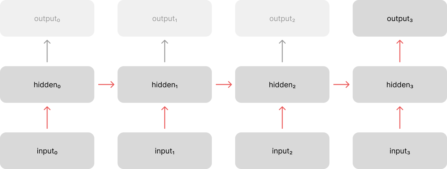
The above visualization shows the "unrolled" representation of our network, but if we were to look at a single time step it becomes more clear that we're only processing the immediately previous hidden state and the current input.
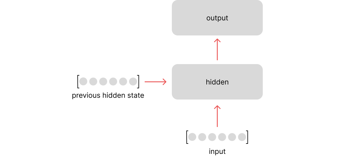
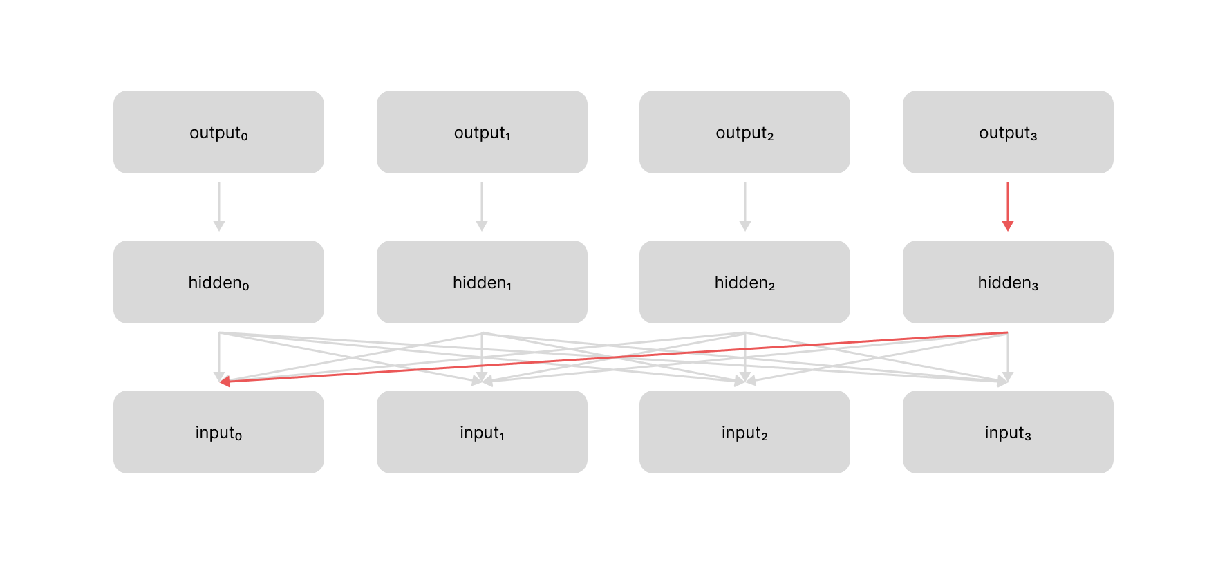
This forces us to evolve a summary of the entire input sequence (represented by the previous hidden state) as we process the sequence step by step. What if we could instead leverage an attention mechanism to look back at every previous time step when building our representation of the current time step?
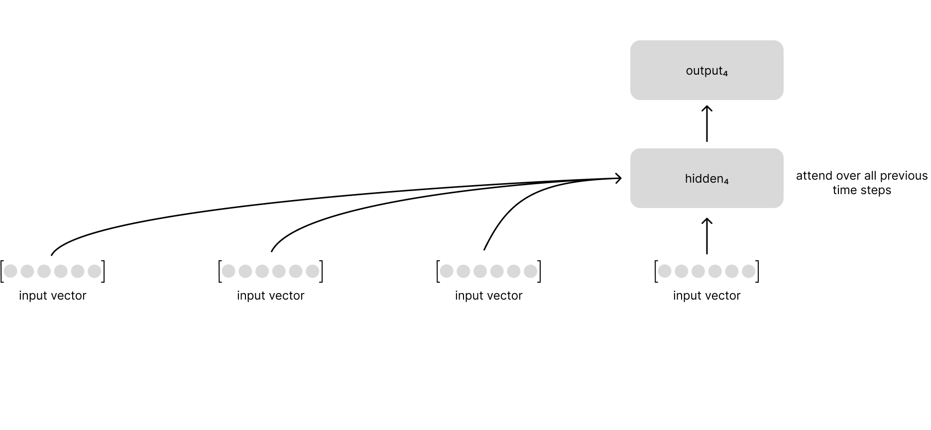
With this approach, we can flexibly look back across the sequence to retrieve relevant information as we process the next item in the input sequence.
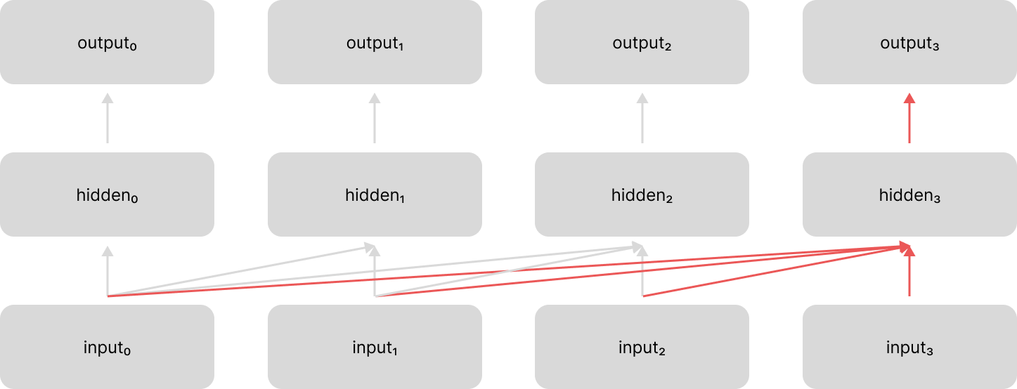
Notice how there is no longer information flowing through the hidden state representation like we had in the unrolled recurrent neural network; in this new architecture, each time-step instead looks back across the entire input sequence.
In some applications, we want to see the entire sequence at each time step, not just the preceding time-steps. With recurrent neural networks we typically achieved this with a bidirectional recurrent layer where we had one recurrent layer processing the input in the forward direction and one recurrent layer processing the input in the backward direction, concatenating these outputs together.
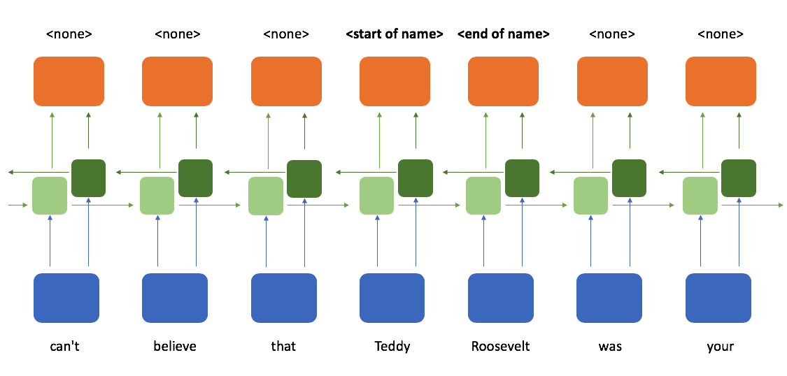
We can achieve this same functionality with an attention-only architecture by simply allowing each time step to attend across all time steps in the sequence.
Further, we can still leverage the attention mechanism for its original design, passing information between an encoder and decoder model. In this case we have attention from two different perspectives:
- self attention: looking across the current sequence being processed (e.g. an encoder network looking across the input sequence being encoded, such as the example shown above)
- cross attention: looking across a related sequence (e.g. the decoder network looking across a sequence of representations from the encoder network)
We describe the type of attention based on the relationship between the sequence that we're currently processing and the sequence that we're using as context.
Generalizing the attention mechanism
With this conceptual understanding in place, let's spend some time digging deeper into how the attention mechanism looks across multiple time steps and combines relevant information into a fixed-size context vector.
At a high level, the attention mechanism:
- compares a reference vector against a candidate vector to determine a relevance score between the two vectors
- performs the above calculation for a set of candidate vectors
- normalizes all of the computed relevance scores (e.g. softmax)
- uses the normalized scores to take a weighted combination of the candidate vectors
This provides us with a single "context" vector which highlights relevant information from across the sequence, relative to the current time-step.
In their paper introducing the Transformer architecture, Vaswani et al refer to the original attention mechanism implementation as "additive attention" and compare this to another proposed mechanism known as "dot-product (multiplicative) attention". The authors then build on this second mechanism to introduce a variant known as "scaled dot product attention". Let's discuss these various implementations and show how they relate to the high-level structure presented above.
Additive attention
I previously introduced the attention model as a small neural network which maps $\left[ \text{reference} ,\ \text{candidate} \right] \rightarrow \text{relevance score}$ where our input is a concatenation of the reference and candidate vectors.
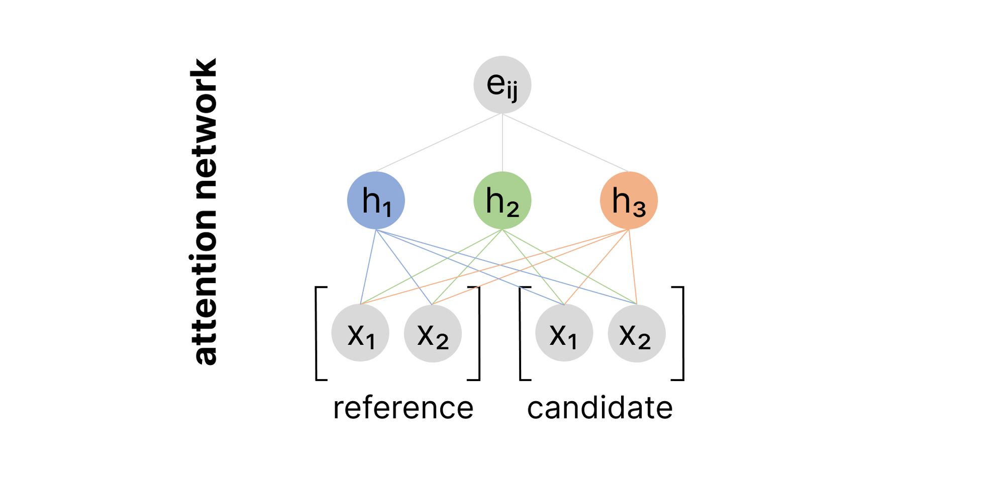
However, instead of concatenating these vectors together and using a single weights matrix to project the input into the hidden layer, we could also project the reference and candidate vectors separately, and then simply add the two projections.
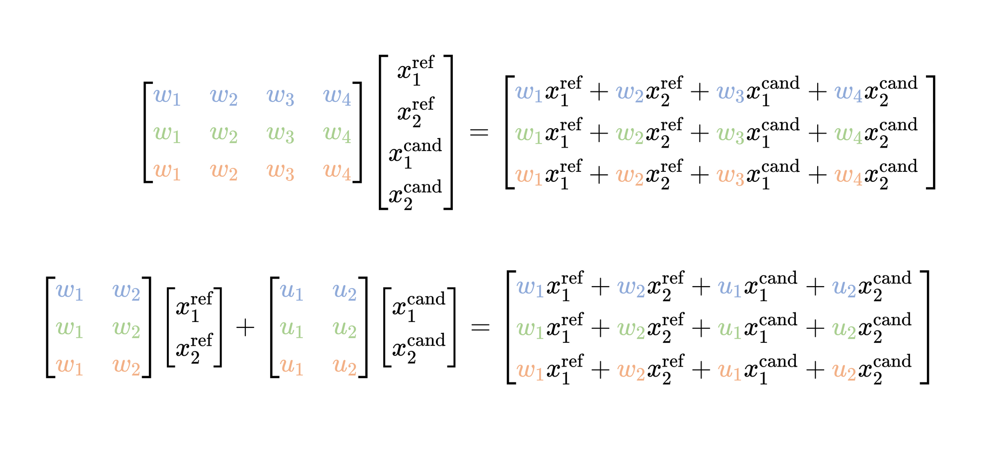
It's advantageous to frame this as two projections which are added together, since the same set of candidate vectors will need to be projected for each reference vector. If we separate these projections, we can cache the results of $Ux^{\text{cand} }$ and reuse this projection in cases where we attend over the same set of candidate vectors multiple times (e.g. cross attention where a decoder autoregressively generates an output sequence and attends over the same sequence of vectors from our encoder representation at each time step).
With this reframing, we will define our additive attention model as:
$$\text{relevance} \left( x^{\text{ref} },\ x^{\text{cand} }\right) =v^{\intercal }\tanh \left( Wx^{\text{ref} }+Ux^{\text{cand} }\right) = e_{i,j}$$
$$\text{attention} \left( x^{\text{ref} },X^{\text{cand} }\right) =\text{softmax} \left( \begin{matrix}e_{i,1}\\ \ldots \\ e_{i,n}\end{matrix} \right) X^{\text{cand} }$$
where $W$ and $U$ are our weights matrices to project from the input to the hidden layer and $v$ represents the weights used to project from the hidden layer to our output. We use $\tanh$ as our nonlinearity in this case but in theory you could swap this out for your nonlinearity of choice.
$X^{\text{cand}}$ denotes our set of candidate vectors as a matrix. These candidate vectors are weighted by the normalized relevance scores and combined to produce our final context vector.
This is the attention model introduced by Bahdanau et al (see appendix section A.1.2) with our inputs renamed to use slightly more generic terminology.
Dot product (multiplicative) attention
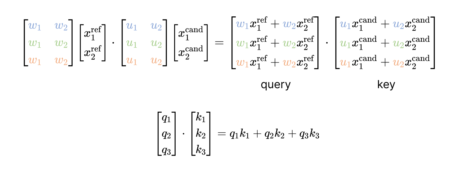
Instead of using a small neural network to compute the relevance score between a reference and candidate vector, a simpler approach might be to take the dot product of the two vectors; this dot product gives us a direct measure of similarity between two vectors. As a quick reminder, the dot product between two vectors is calculated as:
$$\left[ \begin{matrix}a_{1}\\ a_{2}\\ a_{3}\end{matrix} \right] \cdot \left[ \begin{matrix}b_{1}\\ b_{2}\\ b_{3}\end{matrix} \right] =a_{1}b_{1}+a_{2}b_{2}+a_{3}b_{3}$$
If two vectors are aligned in the same direction with similar magnitudes the dot product will be a large positive number. If two vectors are pointing in opposite directions with similar magnitudes, the dot product will be a large negative number. If two vectors are perpendicular, their dot product is zero.
This attention model was originally introduced by Luong et al where attention scores are simply computed by the dot product of our reference and candidate vectors (in their case, the vectors were hidden states of encoder and decoder LSTM networks).
Vaswani et al make a slight modification to this technique, where rather than directly computing the dot product between our reference and candidate vectors, we'll opt to use two learnable weights matrices to project $x^{\text{ref} }$ and $x^{\text{cand} }$ into a new representation subspace, similar to what we did for additive attention.
This transformation into a new representation subspace allows us to extract/highlight information from the input vectors before computing their relevance as determined by the dot product. This also allows us to project the inputs into multiple representation subspaces such that our model can attend to different characteristics of the input in parallel; this is known as multi-headed attention which we'll discuss further in a later section.
Finally, rather than using the candidate vectors directly to perform a weighted combination of our candidate vectors (based on the normalized relevance scores), we'll instead introduce a third projection to use in producing our weighted combination across the candidate vectors.
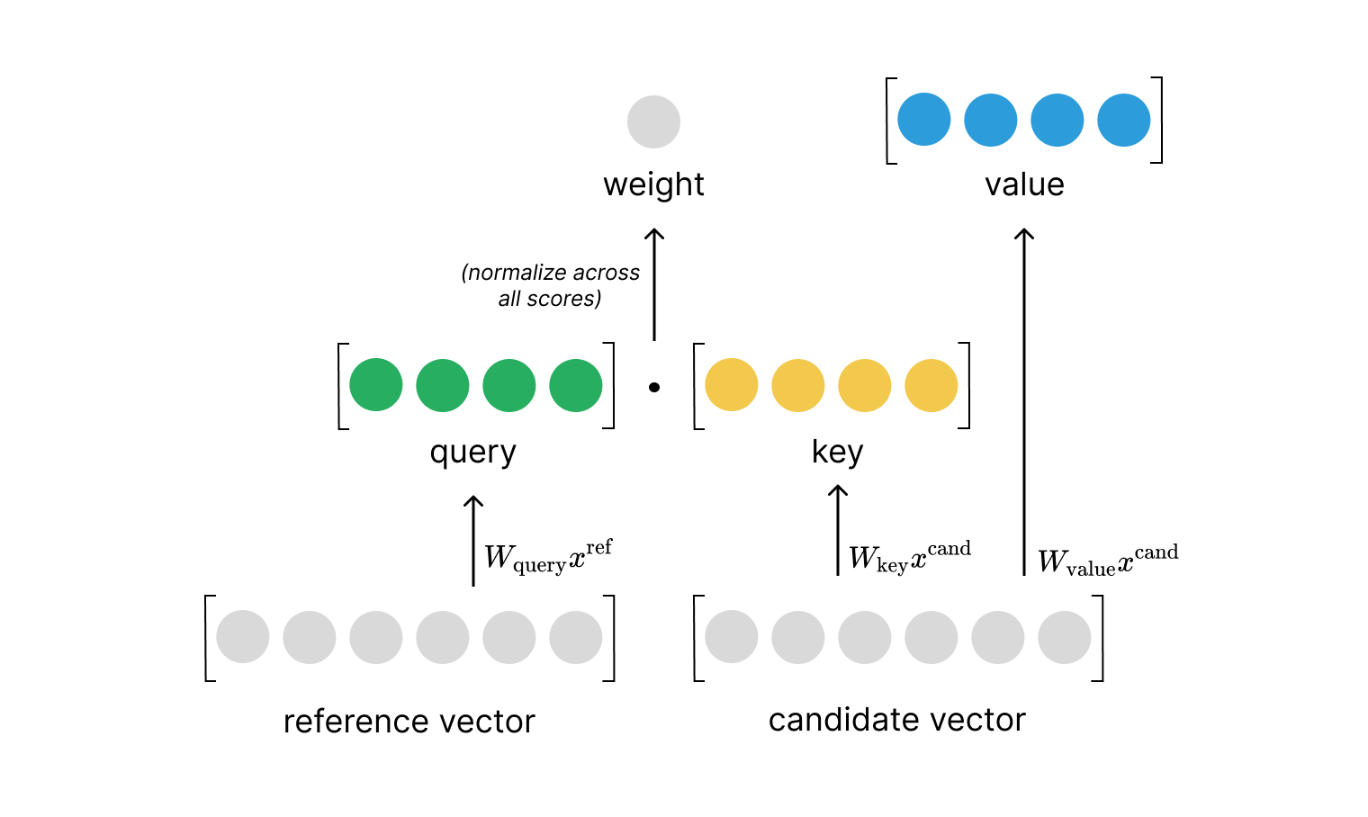
In summary, we'll define dot product attention as:
$$\text{relevance} \left( x^{\text{ref} },\ x^{\text{cand} }\right) =W_{\text{query}}x^{\text{ref} }\cdot W_{\text{key}}x^{\text{cand} }=q\cdot k = e_{i,j}$$
$$\text{attention} \left( x^{\text{ref} },X^{\text{cand} }\right) =\text{softmax} \left( \begin{matrix}e_{i,1}\\ \ldots \\ e_{i,n}\end{matrix} \right) W_{\text{value} }X^{\text{cand} }$$
where our weights matrices $W$ are used to project the input into our query, key, and value vectors and the corresponding relevance scores are denoted as $e_{i,j}$. Here, $i$ denotes our index into a matrix of reference vectors $X^{\text{ref}}$ and $j$ represents the index into the matrix of candidate vectors $X^{\text{cand} }$. For simplicity, we focus the attention calculation on a single reference vector but in practice this can be done in parallel as a single matrix operation treating every vector in our sequence as a reference vector.
Scaled dot product attention
Recall that our relevance scores, $e_{i,j}$, for a given set of candidate vectors are normalized using the softmax function to produce our final attention weights, $a_{i,j}$.
$$a_{i,j}=\frac{\exp \left( e_{i,j}\right)}{\sum^{K}_{k=1}\exp \left( e_{i,k}\right)}$$
Further recall that our dot product between the query and key vectors is computed as $q_{1}k_{1}+q_{2}k_{2}+\ldots +q_{d}k_{d}$. If we were to assume that our two vectors were normally distributed (mean of 0 and variance of 1), we would expect their dot product to have a mean of 0 and a variance of $d$. Thus, as the dimensionality $d$ grows larger, so does the variance of the dot product.
Unfortunately, large magnitudes of our relevance scores push the softmax function into regions of extremely small gradients, which attenuates our learning signal during training. To counteract this effect, Vaswani et al opt to scale the dot products by $\frac{1}{\sqrt{d_{k}} }$ before normalizing them with the softmax function.
With this variant of attention, we compute the relevance score as
$$\text{relevance} \left( x^{\text{ref} },\ x^{\text{cand} }\right) =\frac{1}{\sqrt{d_{k}} } \left( W_{\text{query} }x^{\text{ref} }\cdot W_{\text{key} }x^{\text{cand} }\right) =\frac{1}{\sqrt{d_{k}} } \left( q\cdot k\right)$$
where $d_{k}$ denotes the dimensionality of our query and key vectors.
Putting this all together, we can visualize a scaled dot product attention layer using self-attention to process a sequence of inputs. This visual just shows the computation to produce the context vector for the first time step in the sequence, but you can imagine a similar computation happening in parallel for all time steps.
Defining the Transformer architecture
Let's now discuss the Transformer architecture as presented by Vaswani et al. This architecture was constructed for the task of machine translation and leverages the typical encoder-decoder approach where the encoder processes a sentence in the input language and the decoder uses representations from the encoder to generate a sentence in the target language.
The overall Transformer architecture is mainly a composition and stacking of just a few building blocks:
- scaled dot product attention,
- residual connections,
- layer normalization,
- and feed forward networks.
Stacking multiple attention layers on top of each other has the effect of increasing the receptive field. The first attention layer produces context vectors based on interactions between pairs from the original sequence. The second attention layer produces context vectors based on pairs of pairs of the original sequence. As we continue to stack more attention layers on top of each other, we gain a wider perspective considering multiple levels of interactions between items in the original sequence.
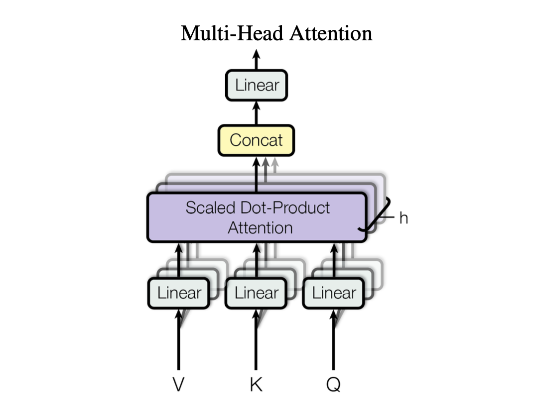
Multi-head attention
For the attention layers, the authors leverage a multi-headed attention implementation where we perform multiple queries in parallel for each time step.
With this approach, we end up with a set of context vectors at each time step in the sequence. These context vectors represent different attention summaries of the same sequence which provides us with multiple perspectives on the same input. The vectors are then concatenated together and passed through a final linear layer.
Encoder
An encoder block is defined as:
- multi-head (self) attention: queries are computed for each step in the input sequence and are compared against keys computed across all steps in the input sequence
- residual connection and layer normalization: the input embeddings are added to context vectors produced from the self-attention layer to create a residual connection, and normalized across the layer dimension (e.g. the output vectors for each sequence in the batch will be separately normalized to have zero mean and unit variance)
- feed forward: we then pass the normalized output from our attention sublayer through a linear projection, ReLU activation, and another linear projection
- residual connection and layer normalization: finally, we add the projection from the feed forward sublayer to the normalized output from our attention sublayer, and once again normalize this vector to have zero mean and unit variance
The encoder model is comprised of 6 of these blocks stacked on top of each other.
Decoder
A decoder block is defined as:
- multi-head (masked self) attention: queries are computed for each step in the output sequence and are compared against keys computed across all steps in the output sequence, due to the fact output sequence is intended to be generated autoregressively we apply a causal mask to the computed relevance scores (limiting the model to only attend across previous time steps)
- residual connection and layer normalization: the embeddings of our output sequence are added to context vectors produced from the causal self-attention layer to create a residual connection, and normalized across the layer dimension
- multi-head (cross) attention: we use the output of the previous self-attention sublayer to generate a second set of queries for each step in the output sequence, the keys and values are computed from the output of the final encoder block across all steps in the input sequence
- residual connection and layer normalization: the context vectors from the causal self-attention sublayer are added to context vectors produced from the cross-attention sublayer to create a residual connection, and normalized across the layer dimension
- feed forward: we then pass the normalized output from our attention sublayer through a linear projection, ReLU activation, and another linear projection
- residual connection and layer normalization: finally, we add the projection from the feed forward sublayer to the normalized output from our cross-attention sublayer, and once again normalize this vector to have zero mean and unit variance
The decoder model is comprised of 6 of these blocks stacked on top of each other.
Embeddings
Our input and output sequences are ultimately represented as a sequence of token ids (integers). To prepare these sequences for our model, we will leverage the standard technique of using this token id as an index to look up a vector of learnable parameters from an embeddings matrix. However, we must also inject some additional information into these embeddings so that the model can learn positional relationships between tokens in our input and output sequences.
This is because the attention mechanism doesn't have any notion of spatial relationships between tokens in the sequence. Our query at each time step simply looks across the set of keys and determines which keys are most relevant to our current time step; if we shuffled up the order of the sequence this would have no effect on our pairwise relevance comparisons.
However, we know intuitively that token order should matter, so the authors develop a technique known as positional encoding to inject information about the order of the tokens in our sequence.
We encode the position $pos$ in a sequence using a combination of $sin$ and $cos$ functions (alternating these functions for each dimension $i$ in the $d$-dimensional embedding vector).
$$PE_{\left( pos,2i\right) }=sin(\frac{pos}{10000^{\frac{2i}{d} }} )$$
$$PE_{\left( pos,2i+1\right) }=cos(\frac{pos}{10000^{\frac{2i}{d} }} )$$
These position encodings are then added to our embedding vectors before being passed to the encoder or decoder models.
Overall architecture
Putting all this together, we have the Transformer architecture.
Benefits of an attention-only architecture
One of the biggest benefits of replacing recurrence with attention is that we now have a fully parallelizable architecture. Whereas recurrence requires us to process a sequence one time-step at a time (due to the fact that we rely on the previous hidden state to process the next item in a sequence), an attention-only architecture does not have such a limitation. You can use a single matrix operation to project queries, keys, and values for every time-step in your sequence, simultaneously attending across the sequence for every time-step in parallel. This allows us to more efficiently leverage accelerated compute infrastructure (e.g. GPUs) and train models faster.
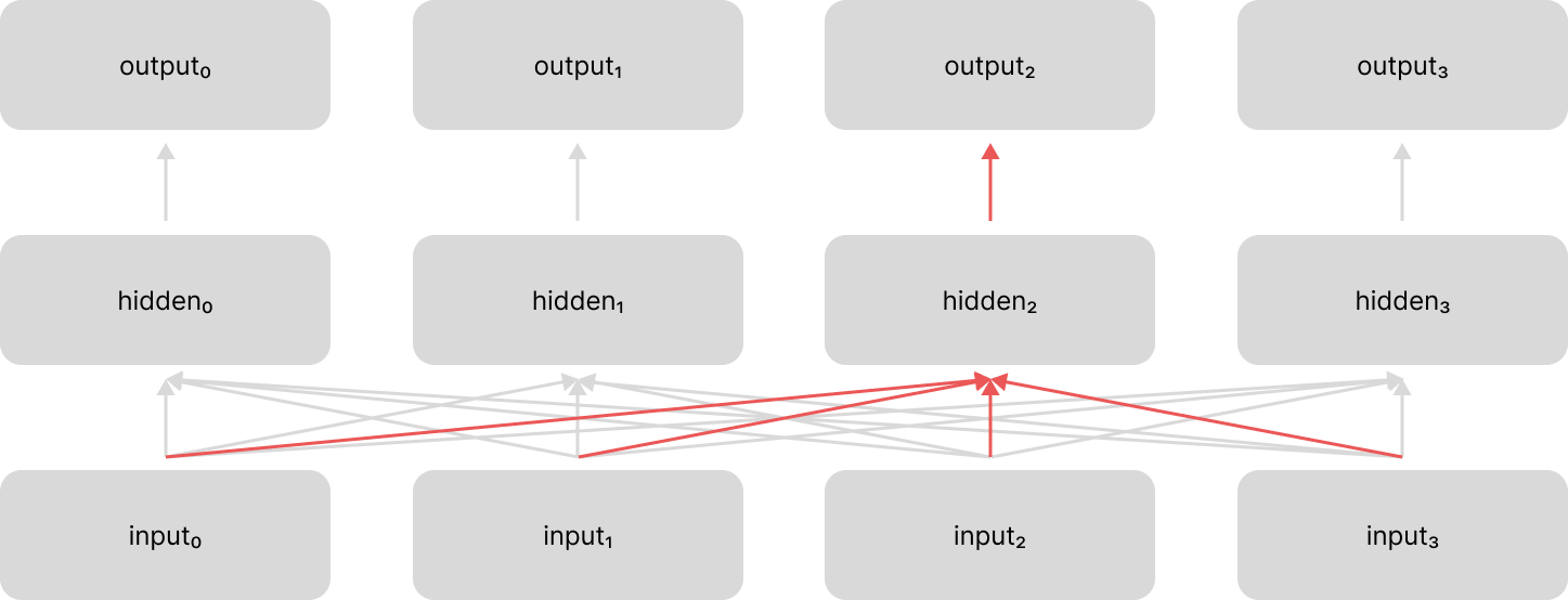
The attention mechanism also allows our gradient signal to flow through the network more efficiently during backpropagation. With recurrent neural networks, if you needed propagate a gradient signal from $t=3$ back to $t=0$, you would have to back-propagate through all of the recurrent hidden layers between each of these time-steps.
However, with the attention mechanism we can directly back-propagate our gradient signal across an arbitrarily number of time steps using a constant number of operations.
These shorter path lengths make it easier for the model to learn long-term dependencies between items in our sequence.
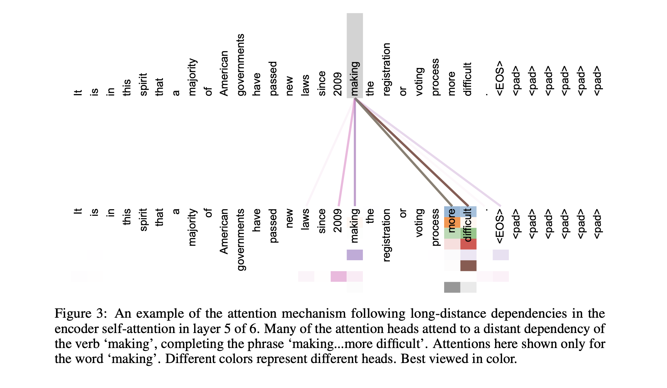
Finally, the attention mechanism has an inherent level of interpretability as a result of inspecting the attention weights. That is, we can use the computed attention weights to understand which tokens across the sequence were deemed relevant and used to produce a context vector for any given token in the sequence.
Resources
Papers
- Neural Machine Translation by Jointly Learning to Align and Translate
- Effective Approaches to Attention-based Neural Machine Translation
- Attention Is All You Need 🐐
- On Layer Normalization in the Transformer Architecture
- Train Short, Test Long: Attention with Linear Biases Enables Input Length Extrapolation (replace positional encoding)
- The author gives a nice overview of the paper in this talk
Lectures
- 3Blue1Brown Series
- Sebastian Raschka's lectures on this topic
- Andrej Karpathy's deep dive + live coding
Blog posts
- The Illustrated Transformer
- The Annotated Transformer
- Understanding and Coding the Self-Attention Mechanism of Large Language Models From Scratch
- A walkthrough of transformer architecture code
Other
- Calculus (OpenStax) 12.3: The Dot Product
- LLM Visualization
- This is a really impressive interactive visualization.
Thanks to James Black, Tim Hopper, and ChatGPT for pointing me to ffmpeg and helping me figure out the right settings to use to create GIFs from my diagrams. I hope you found the animations to be useful!