Introduction to recurrent neural networks.
In this post, I'll discuss a third type of neural networks, recurrent neural networks, for learning from sequential data. For some classes of data, the order in which we receive observations is important. As an example, consider the two following sentences:

Jump to:
- Overview
- Evolving a hidden state over time
- Common structures of recurrent networks
- Bidirectionality
- Limitations
- Further reading
Overview
Previously, I've written about feed-forward neural networks as a generic function approximator and convolutional neural networks for efficiently extracting local information from data. In this post, I'll discuss a third type of neural networks, recurrent neural networks, for learning from sequential data.
For some classes of data, the order in which we receive observations is important. As an example, consider the two following sentences:
- "I'm sorry... it's not you, it's me."
- "It's not me, it's you... I'm sorry."
These two sentences are communicating quite different messages, but this can only be interpreted when considering the sequential order of the words. Without this information, we're unable to disambiguate from the collection of words: {'you', 'sorry', 'me', 'not', 'im', 'its'}.
Recurrent neural networks allow us to formulate the learning task in a manner which considers the sequential order of individual observations.
Evolving a hidden state over time
In this section, we'll build the intuition behind recurrent neural networks. We'll start by reviewing standard feed-forward neural networks and build a simple mental model of how these networks learn. We'll then build on that to discuss how we can extend this model to a sequence of related inputs.
Recall that neural networks perform a series of layer by layer transformations to our input data. The hidden layers of the network form intermediate representations of our input data which make it easier to solve the given task.
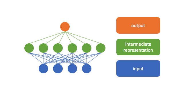
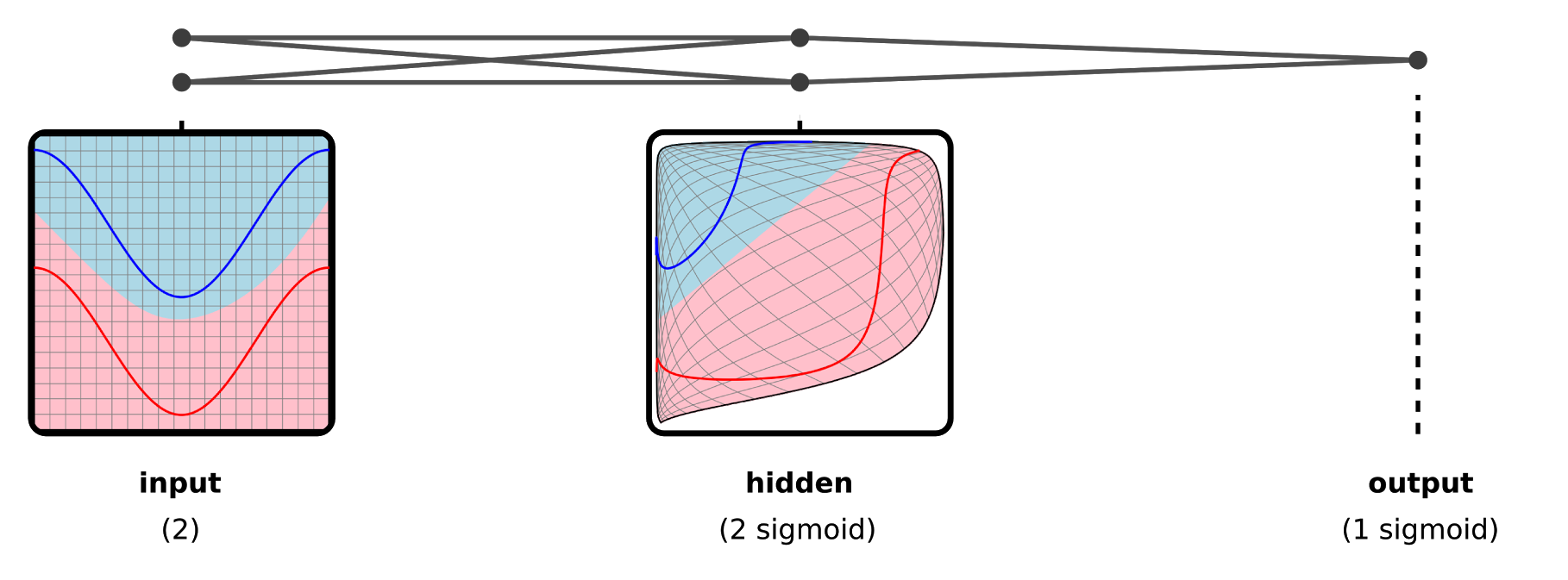
This is demonstrated in the example below. Observe how our input space is warped into one which allows for a linear decision boundary to cleanly separate the two classes. At a high level, you can think of the hidden layers as "useful representations" of the original input data.
Now let's consider how we can leverage this insight for a sequence of related observations.
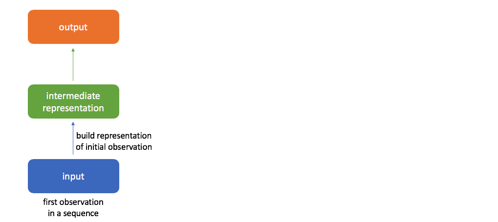
Let's first focus on the initial value in the sequence. As we calculate the forward pass through the network, we build a "useful representation" of our input in the hidden layers (the activations in these layers define our hidden state), continuing on to calculate an output prediction for the initial time-step.
When considering the next time-step in the sequence, we want to leverage any information we've already extracted from the sequence.
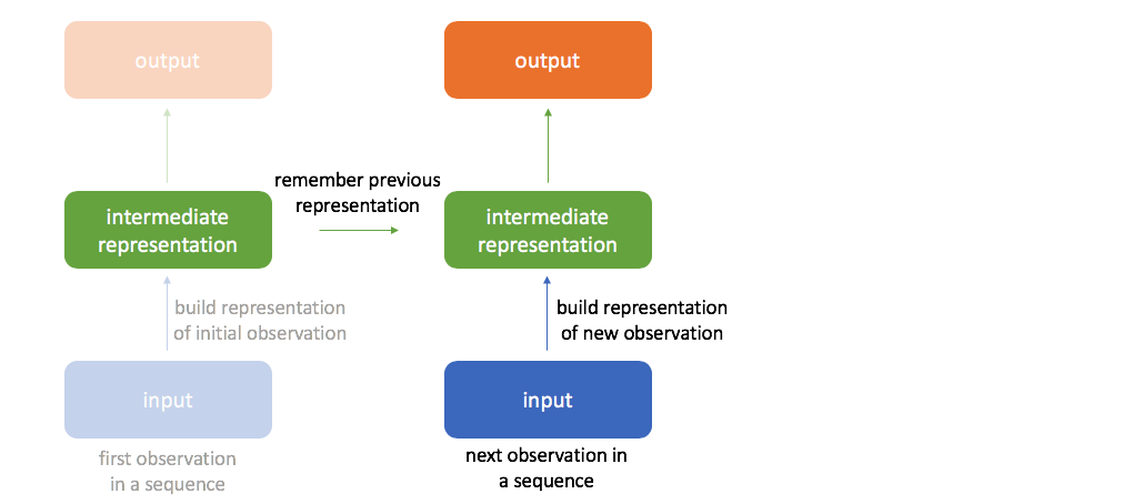
In order to do this, our next hidden state will be calculated as a combination of the previous hidden state and latest input.
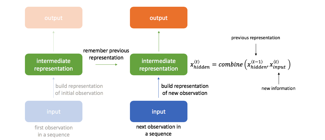
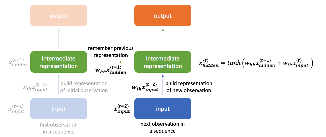
The basic method for combining these two pieces of information is shown below; however, there exist other more advanced methods that we'll discuss later (gated recurrent units, long short-term memory units). Here, we have one set of weights $w_{ih}$ to transform the input to a hidden layer representation and a second set of weights $w_{hh}$ to bring along information from the previous hidden state into the next time-step.
We can continue performing this same calculation of incorporating new information to update the value of the hidden state for an arbitrarily long sequence of observations.
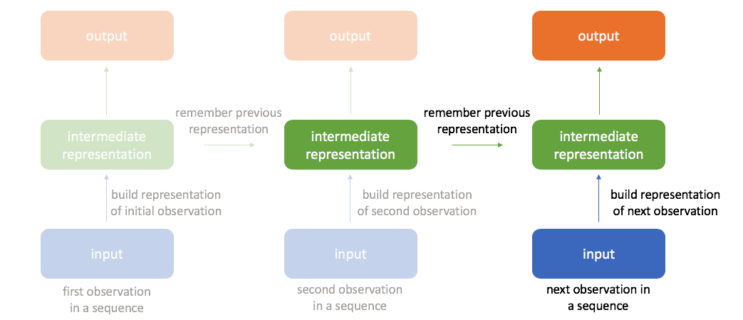
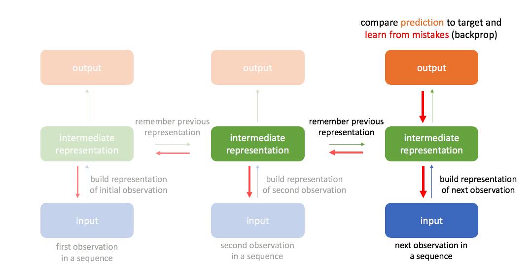
By always remembering the previous hidden state, we're able to chain a sequence of events together. This also allows us to backpropagate errors to earlier timesteps during training, often referred to as "backpropagation through time".
Common structures of recurrent networks
One of the benefits of recurrent neural networks is the ability to handle arbitrary length inputs and outputs. This flexibility allows us to define a broad range of tasks. In this section, I'll discuss the general architectures used for various sequence learning tasks.
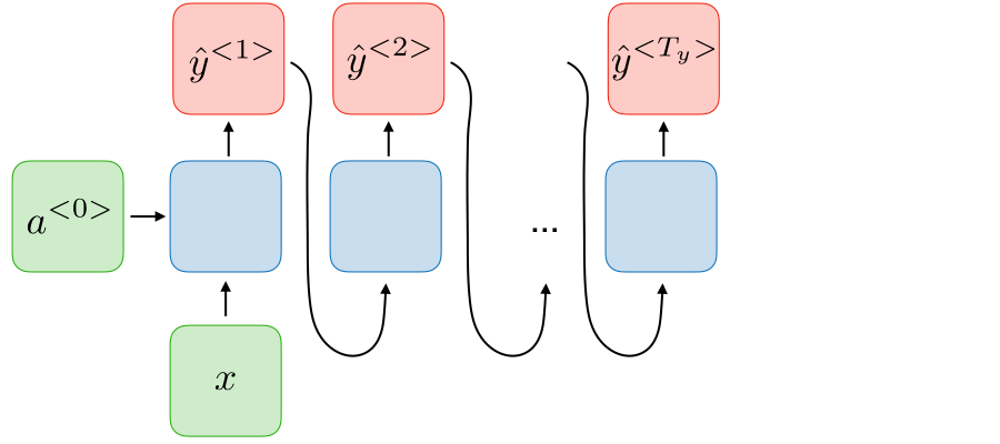
One to many RNNs are used in scenarios where we have a single input observation and would like to generate an arbitrary length sequence related to that input. One example of this is image captioning, where you feed in an image as input and output a sequence of words to describe the image. For this architecture, we take our prediction at each time step and feed that in as input to the next timestep, iteratively generating a sequence from our initial observation and following predictions.
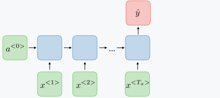
Many to one RNNs are used to look across a sequence of inputs and make a single determination from that sequence. For example, you might look at a sequence of words and predict the sentiment of the sentence. Generally, this structure is used when you want to perform classification on sequences of data.
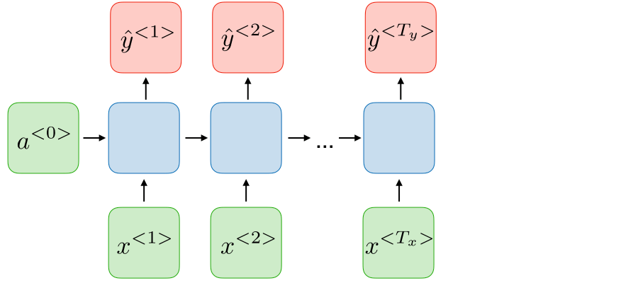
Many to many (same) RNNs are used for tasks in which we would like to predict a label for each observation in a sequence, sometimes referred to as dense classification. For example, if we would like to detect named entities (person, organization, location) in sentences, we might produce a label for every single word denoting whether or not that word is part of a named entity. As another example, you could feed in a video (sequence of images) and predict the current activity in frame.
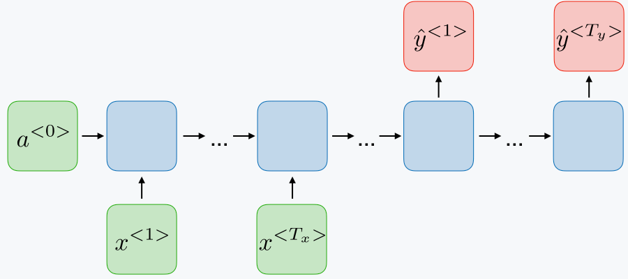
Many to many (different) RNNs are useful for translating a sequence of inputs into a different but related sequence of outputs. In this case, both the input and the output can be arbitrary length sequences and the input length might not always be equal to the output length. For example, a machine translation model would be expected to translate "how are you" (input) into "cómo estás" (output) even though the sequence lengths are different.
Bidirectionality
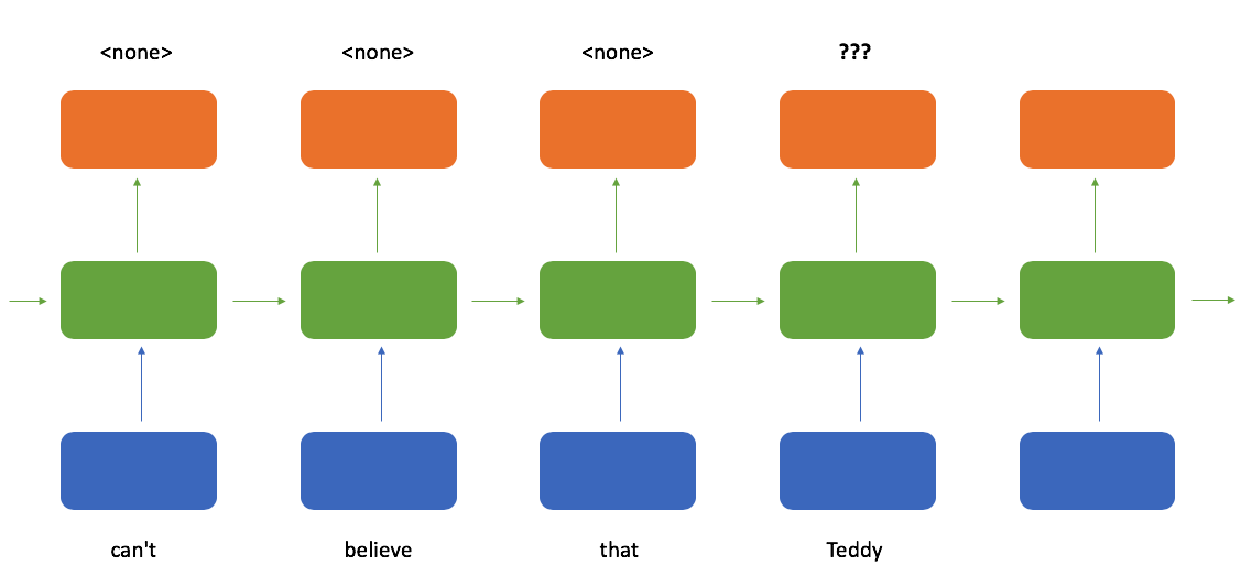
One of the weaknesses of a ordinary recurrent neural networks is that we can only use the set of observations which we have already seen when making a prediction. As an example, consider training a model for named entity recognition. Here, we want the model to output the start and end of phrases which contain a named entity. Consider the following two sentences:
"I can't believe that Teddy Roosevelt was your great grandfather!"
"I can't believe that Teddy bear is made out of chocolate!"
However, if you only read the input sequence from left to right, it's hard to tell whether or not you should mark "Teddy" as the start of a name.
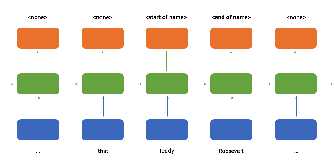
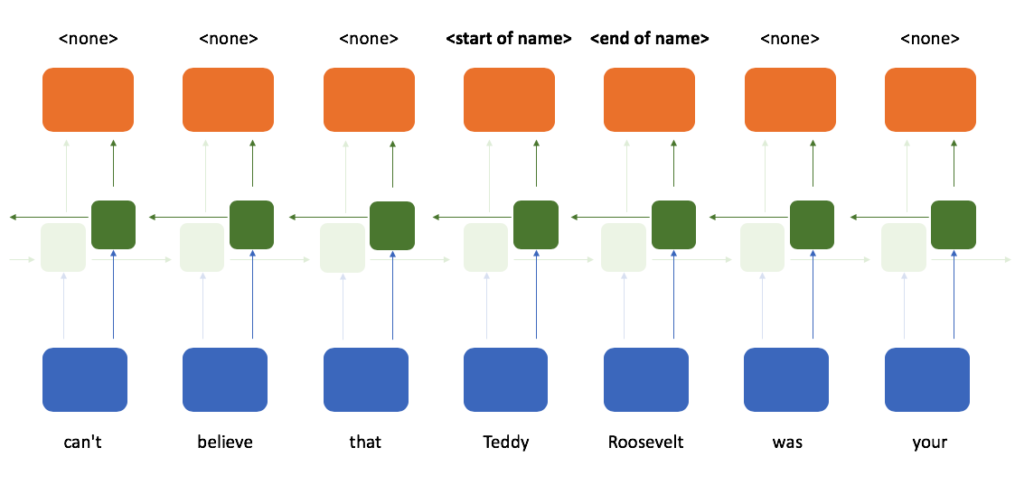
Ideally, our model output would look something like this when reading the first sentence (roughly following the inside–outside–beginning tagging format).
When determining whether or not a token is the start of a name, it would sure be helpful to see which tokens follow after it; a bidirectional recurrent neural network provides exactly that. Here, we process the sequence reading from left-to-right and right-to-left in parallel and then combine these two representations such that at any point in a sequence you have knowledge of the tokens which came before and after it.
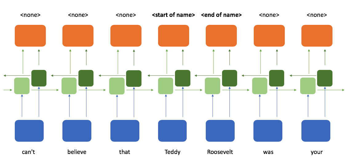
We have one set of recurrent cells which process the sequence from left to right...
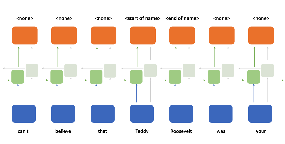
... and another set of recurrent cells which process the sequence from right to left.
Thus, at any given time-step we have knowledge of all of the tokens which came before the current time-step and all of the tokens which came after that time-step.
Limitations
One key component that I glanced over previously is that the recurrent layer's weights are shared across time-steps. This provides us with the flexibility to process arbitrary length sequences, but also introduces a unique challenge when training the network.
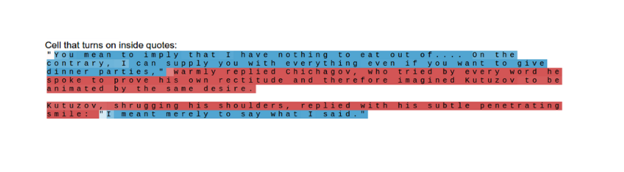
For a concrete example, suppose you've trained a recurrent neural network as a language model (predict the next word in a sequence). As you're generating text, it might be important to know whether the current word is inside quotation marks. Let's assume this is true and consider the case where our model makes a wrong prediction because it wasn't paying attention to whether or not the current time-step is inside quotation marks. Ideally, you want a way to send back a signal to the earlier time-step where we entered the quotation mark to say "pay attention!" to avoid the same mistake in the future. Doing so requires sending our error signal back through many time-steps. (As an aside, Karpathy has a famous blog post which shows that a character-level RNN language model can indeed pay attention to this detail.)
Let's consider what the backpropagation step would look like to send this signal to earlier time-steps.
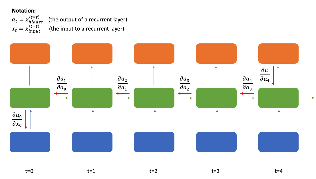
As a reminder, the backpropagation algorithm states that we can define the relationship between a given layer's weights and the final loss using the following expression:
$$ \frac{{\partial E\left( w \right)}}{{\partial w^{(l)}}} = {\left( {{\delta ^{(l + 1)}}} \right)^T}{a^{(l)}} $$
where ${\delta ^{(l)}}$ (our "error" term) can be calculated as:
$$ {\delta ^{(l)}} = {\delta ^{(l + 1)}}{w ^{(l)}}f'\left( {{a^{(l)}}} \right) $$
This allows to efficiently calculate the gradient for any given layer by reusing the terms already computed at layer $l+1$. However, notice how there's a term for the weight matrix, ${w ^{(l)}}$, included in the computation at every layer. Now recall that I earlier mentioned recurrent layers share weights across time-steps. This means that the same exact value is being mulitplied every time we perform this layer by layer backpropagation through time.
Let's suppose one of the weights in our matrix is 0.5 and we're attempting to send a signal back 10 time-steps. By the time we've backpropagated to $t-10$, we've multiplied the overall gradient expression by $0.5 \cdot 0.5 \cdot 0.5 \cdot 0.5 \cdot 0.5 \cdot 0.5 \cdot 0.5 \cdot 0.5 \cdot 0.5 \cdot 0.5 = 0.00098$. This has the effect of drastically reducing the magnitude of our error signal! This phenomenon is known as the "vanishing gradient" problem which makes it very hard to learn using a vanilla recurrent neural network. The same problem can occur when the weight is greater than one, introducing an exploding gradient, although this is slightly easier to manage thanks to a technique known as gradient clipping.
In following posts, we'll look at two common variations of the standard recurrent cell which alleviate this problem of a vanishing gradient.
Further reading
Papers
- Learning Long-Term Dependencies with Gradient Descent is Difficult
- On the difficulty of training Recurrent Neural Networks
- A Simple Way to Initialize Recurrent Networks of Rectified Linear Units
Lectures/Notes
- Stanford CS231n: Lecture 10 | Recurrent Neural Networks
- Stanford CS231n Winter 2016: Lecture 10: Recurrent Neural Networks, Image Captioning, LSTM
- Stanford CS224n: Lecture 8: Recurrent Neural Networks and Language Models
- Stanford CS230: Recurrent Neural Networks Cheatsheet
- MIT 6.S094: Recurrent Neural Networks for Steering Through Time
- University of Toronto CSC2535: Lecture 10 | Recurrent neural networks
Blog posts