Convolutional neural networks.

In my introductory post on neural networks, I introduced the concept of a neural network that looked something like this.
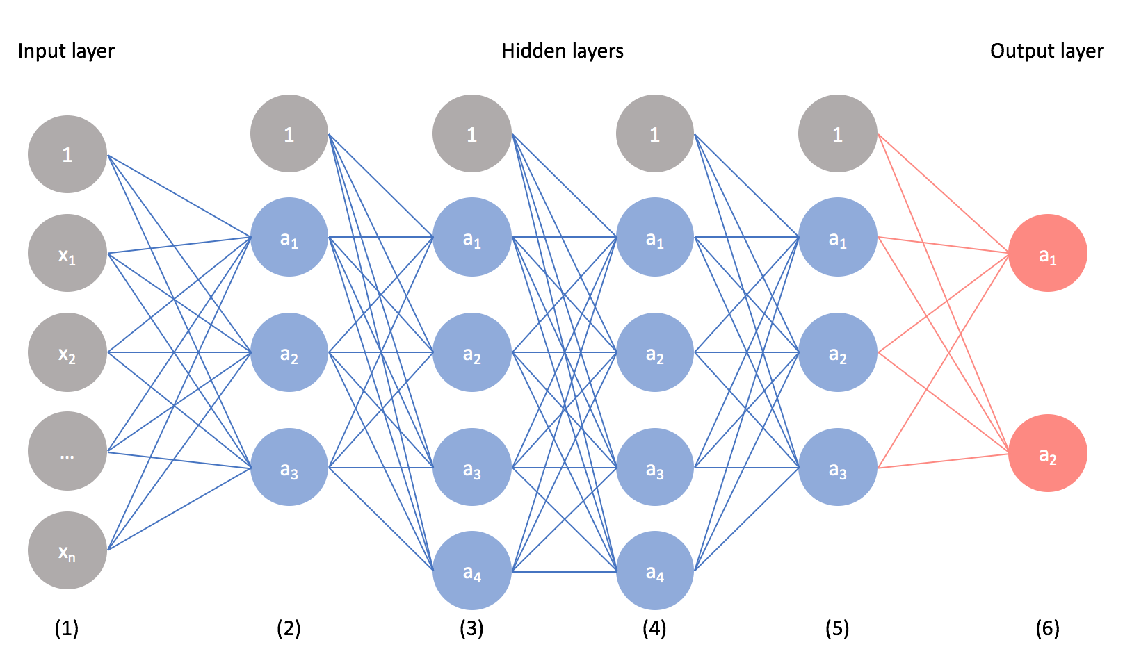
As it turns out, there are many different neural network architectures, each with its own set of benefits. The architecture is defined by the type of layers we implement and how layers are connected together. The neural network above is known as a feed-forward network (also known as a multilayer perceptron) where we simply have a series of fully-connected layers.
Today, I'll be talking about convolutional neural networks which are used heavily in image recognition applications of machine learning. Convolutional neural networks provide an advantage over feed-forward networks because they are capable of considering locality of features.
Consider the case where we'd like to build an neural network that could recognize handwritten digits. For example, given the following 4 by 4 pixel image as input, our neural network should classify it as a "1".
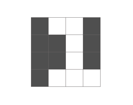
Images are simply a matrix of values corresponding with the intensity of light (white for highest intensity, black for lowest intensity) at each pixel value. Grayscale images have a single value for each pixel while color images are typically represented by light intensity values for red, green, and blue at each pixel value. Thus, a 400 by 400 pixel image has the dimensions $\left[ {400 \times 400 \times 1} \right]$ for a grayscale image and $\left[ {400 \times 400 \times 3} \right]$ for a color image. When using images for machine learning models, we'll typically rescale the light intensity values to be bound between 0 and 1.
Revisiting feed-forward networks
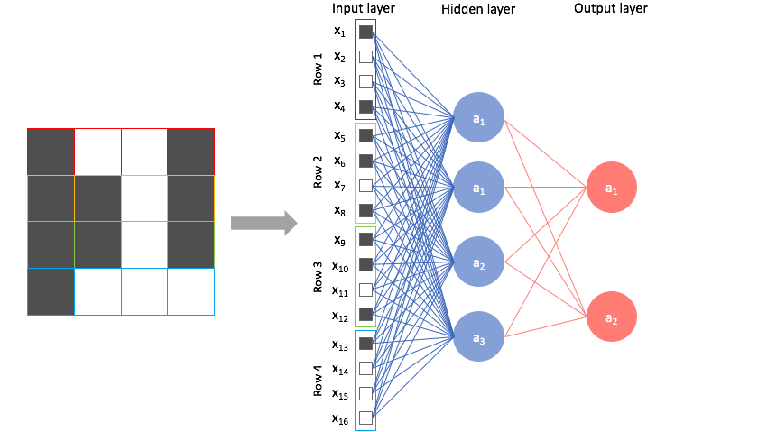
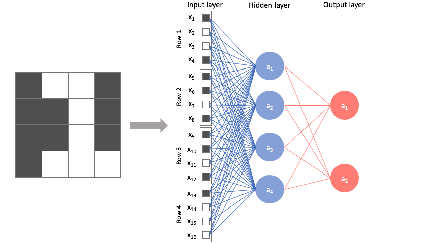
First, let's examine what this would look like using a feed-forward network and identify any weaknesses with this approach. Foremost, we can't directly feed this image into the neural network. A feed-forward network takes a vector of inputs, so we must flatten our 2D array of pixel values into a vector.
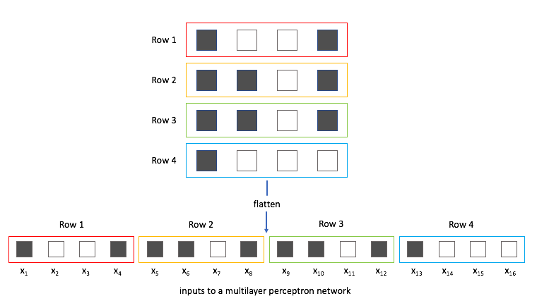
Now, we can treat each individual pixel value as a feature and feed it into the neural network.
Unfortunately, we lose a great deal of information about the picture when we convert the 2D array of pixel values into a vector; specifically, we lose the spatial relationships within the data.
Just ask yourself, could you identify the following numbers in flattened vector form without rearranging the pixels back into a 2D array in your head?
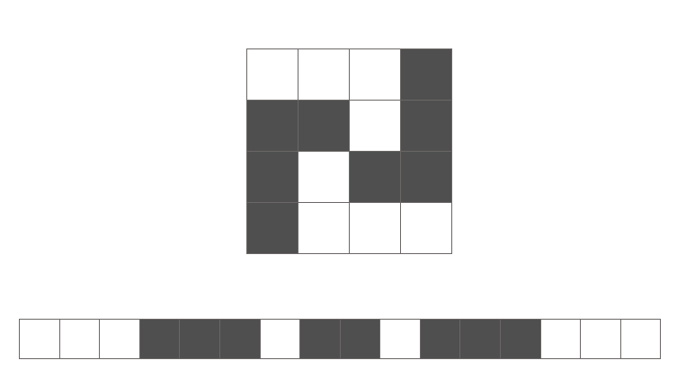
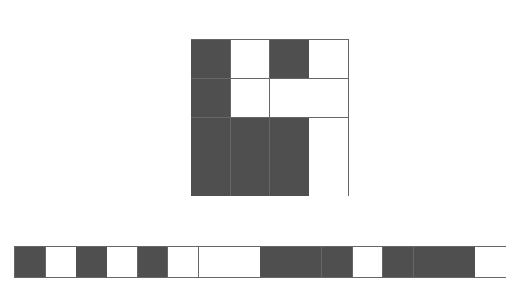
Don't kid yourself, you can't. The spatial arrangement of features (pixels) is important because we see in a relativistic perspective. This is where convolutional neural networks shine.
Convolution layers
A convolution layer defines a window by which we examine a subset of the image, and subsequently scans the entire image looking through this window. As you'll see below, we can parameterize the window to look for specific features (e.g. edges) within an image. This window is also sometimes called a filter, since it produces an output image which focuses solely on the regions of the image which exhibited the feature it was searching for. The output of a convolution is referred to as a feature map.
Note: Windows, filters, and kernels all refer to the same thing with respect to convolutional neural networks; don't get confused if you see one term being used instead of another.
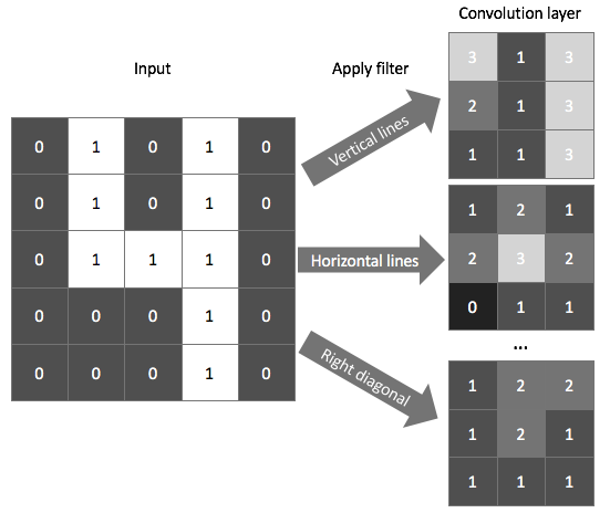
For example, the following window searches for vertical lines in the image.
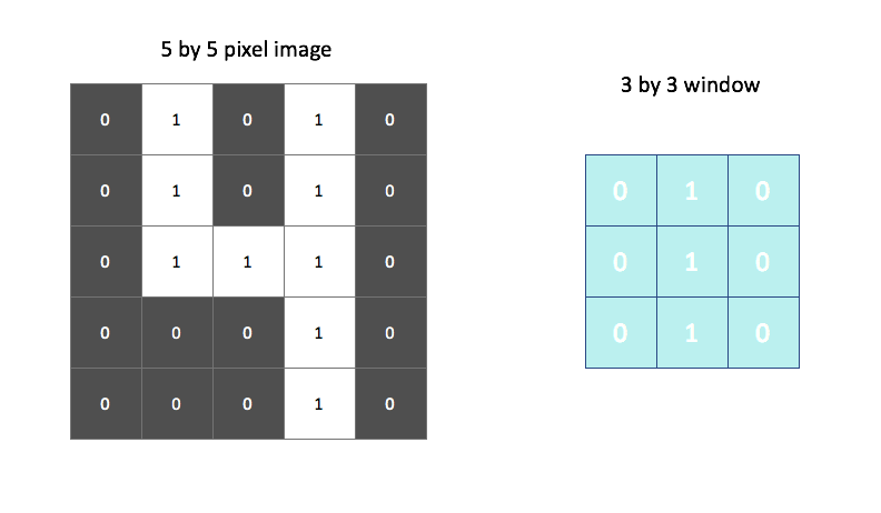
We overlay this filter onto the image and linearly combine (and then activate) the pixel and filter values. The output, shown on the right, identifies regions of the image in which a vertical line was present. We could do a similar process using a filter designed to find horizontal edges to properly characterize all of the features of a "4".
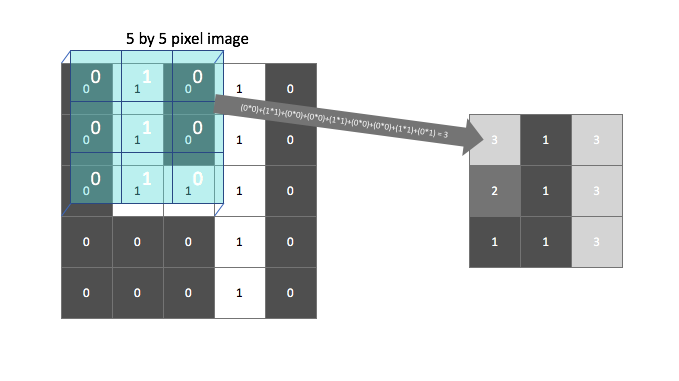
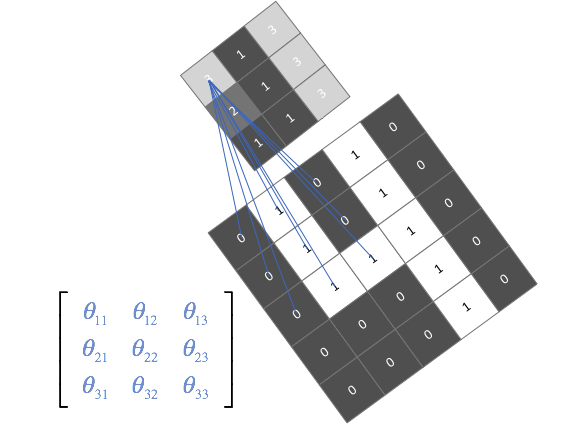
We'll scan each filter across the image calculating the linear combination (and subsequent activation) at each step. In the figure below, an input image is represented in blue and the convolved image is represented in green. You can imagine each pixel in the convolved layer as a neuron which takes all of the pixel values currently in the window as inputs, linearly combined with the corresponding weights in our filter.
You can also pad the edges of your images with 0-valued pixels as to fully scan the original image and preserve its complete dimensions.

Image credit
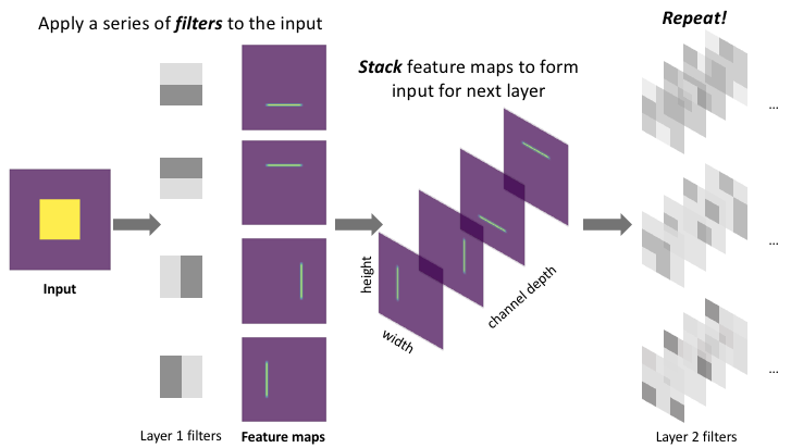
As an example, I took an image of myself sailing and applied four filters, each of which look for a certain type of edge in the photo. You can see the resulting output below.
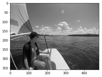
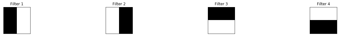
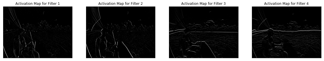
As shown in the example above, a typical convolutional layer will apply multiple filters, each of which output a feature mapping of the input signifying the (spatial) locations where a feature is present. Notice how some feature mappings are more useful than others; in the below example, the "right diagonal" feature mapping, which searches for right diagonals in the image, is essentially a dark image which signifies that the feature is not present.
In practice, we don't explicitly define the filters that our convolutional layer will use; we instead parameterize the filters and let the network learn the best filters to use during training. We do, however, define how many filters we'll use at each layer.
We can stack layers of convolutions together (ie. perform convolutions on convolutions) to learn more intricate patterns within the features mapped in the previous layer. This allows our neural network to identify general patterns in early layers, then focus on the patterns within patterns in later layers.
Let's revisit the feed-forward architecture one more time and compare it with convolutional layers now that we have a better understanding of what's going on inside them.
A feed-forward network connects every pixel with each node in the following layer, ignoring any spatial information present in the image.
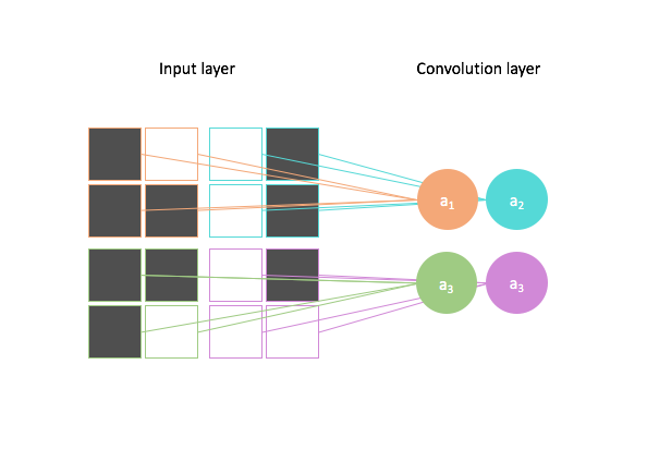
By contrast, a convolutional architecture looks at local regions of the image. In this case, a 2 by 2 filter with a stride of 2 (more on strides below) is scanned across the image to output 4 nodes, each containing localized information about the image.
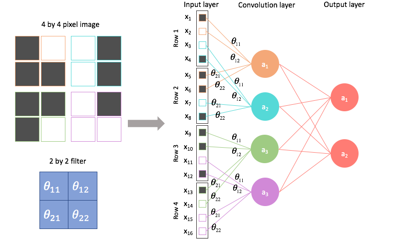
The four nodes can be combined to form the "pixels" of a feature map, where the feature extracted is dependent on the parameters of our filter. Here, spatial information can be preserved.
We can scan the image using multiple filters to generate multiple feature mappings of the image. Each feature mapping will reveal the parts of the image which express the given feature defined by the parameters of our filter.
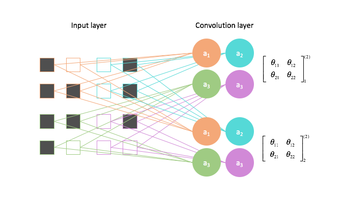
In general, a convolution layer will transform an input into a stack of feature mappings of that input. Depending on how you set your padding, you may or may not reduce the size of your input. The depth of the feature map stack depends on how many filters you define for a layer.
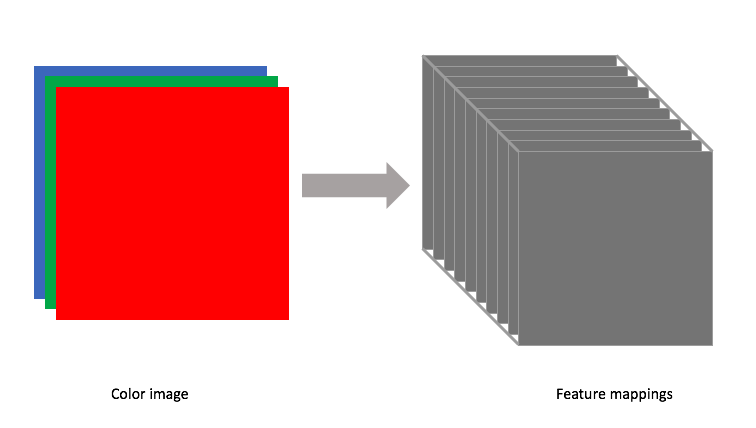
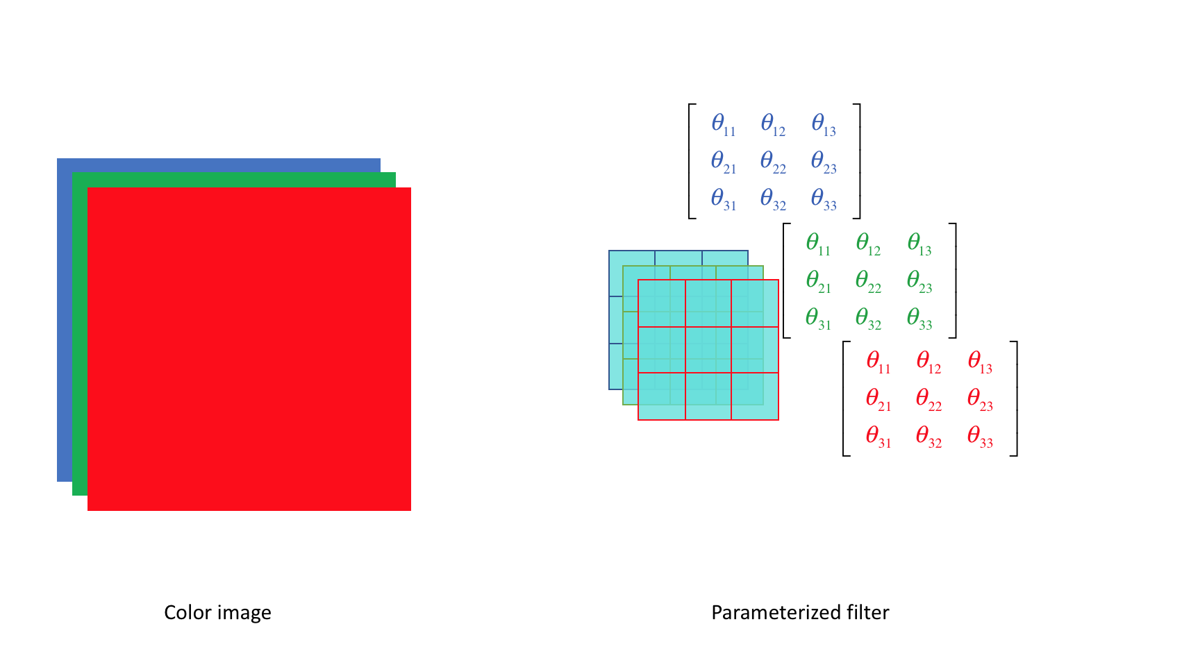
Each filter will have a defined width and height, but the filter depth should match that of the input. For earlier examples where we looked at grayscale images, our filter had a depth=1. However, if we wanted to convolve a color image, for example, we would need a filter with depth=3, containing a filter for each of the three RGB color channels.
Note: The convolution operation may be more accurately describing as calculating the cross correlation between the image input and a given filter. In pure mathematical terms, a convolution involves flipping the kernel matrix, but since we're simply learning parameter values, this operation doesn't add any value.
Deep convolutional networks
I mentioned earlier that we can stack multiple layers of convolutions (each followed by a nonlinear activation) to learn more intricate patterns. I'll now provide a more concrete example of this.
Let's start with a question... how would you describe a square to someone who has never seen the shape before?
Here's one possible answer:
A square is comprised of two sets of parallel lines, all of equal length, which intersect orthogonal to one another.
In this response, we've described the abstract concept of a square using lower-level concepts such as lines and angles. We could use these same lower-level concepts to describe a plethora of shapes.
When we visualize convolutional networks, we find that the same phenomenon occurs. The network learns to use earlier layers to extract low-level features and then combine these features into more rich representations of the data. This means that later layers of the network are more likely to contain specialized feature maps.
Here, I've shown how we could combine successive convolutional operations such that we can detect the presence of a square in the original input. Although I've hard-coded the filter values for this example, the filter values in a convolutional layer are learned.
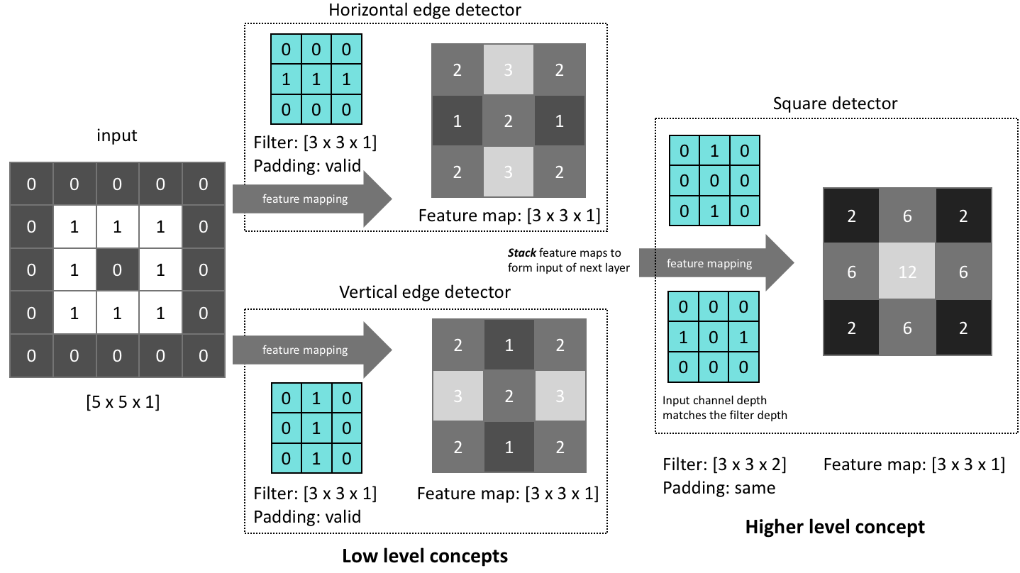
Layers in a convolutional network follow the same general principle, using parameterized filters to transform the input into useful representations.
Reminder: the number of channels in your filter must match the number of channels in your input.
As you progress into deeper layers of a network, it's very common to see an increase in the channel depth (number of feature maps); as feature maps become more specialized, representing higher-level abstract concepts, we simply need more feature maps to represent the input. Consider the fact that a small set of lines can be combined into a large number of shapes, and these shapes can be combined into an even larger number of objects. If our goal is to build a model with general representational power, we'll likely need to grow our feature maps accordingly.
Pooling layers
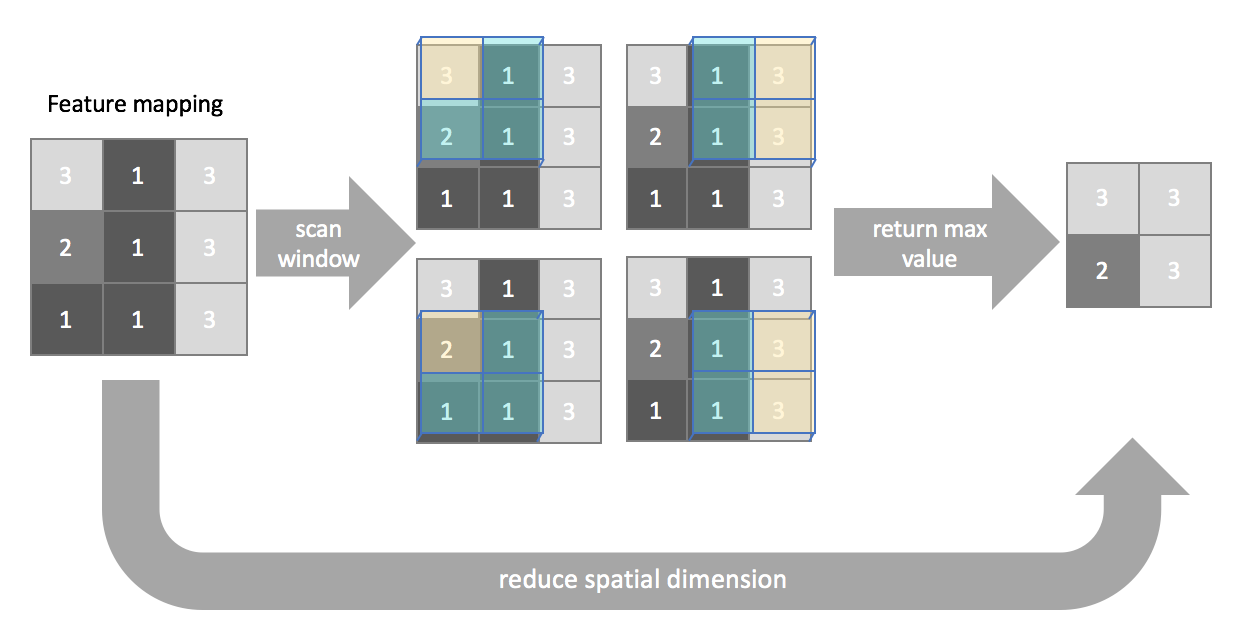
A pooling layer can be used to compress spatial information of our feature mappings. We'll still scan across the image using a window, but this time our goal is to compress information rather than extract certain features. Similar to convolutional layers, we'll define the window size, and stride. Padding is not commonly used for pooling layers.
Max pooling
In max pooling, we simply return the maximum value (highlighted in yellow) present inside the window for each scanning location.
You can similarly define layers for average pooling or minimum pooling when necessary, although max pooling is the most commonly used pooling layer.
Global pooling
Global pooling is a more extreme case, where we define our window to match the dimensions of the input, effectively compressing the size of each feature mapping to a single value. This is useful for building convolutional neural networks in which need to be able to accept a variety of input sizes, as it compresses your feature representation from an arbitrary $w \times h \times c$ into a fixed $1 \times 1 \times c$ feature map.
Strided convolutions
Strided convolutions are an alternative method for downsampling the spatial resolution of our feature mappings which allows for a degree of learned downsampling rather than explicitly defining how to summarize a window (such as the case for max/average/min pooling).
The stride length of a convolution defines how many steps we take when sliding our window (filter) across an image. A standard convolution has a stride length of one, moving the filter one unit as we scan across the input.
Alternatively, if we were to define a stride length of two, we would move the filter by two units for each calculation.
Notice how this has the effect of reducing the dimensions of the output feature map, relative to the input.
You can calculate the dimensions of a feature map according to the following formula
$$ \left( {\frac{{{n_{width}} - {f_{width}} + 2{p_{width}}}}{{{s_{width}}}} + 1,\frac{{{n_{height}} - {f_{height}} + 2{p_{height}}}}{{{s_{height}}}} + 1} \right) $$
where $n$ is the input dimension, $f$ is the filter size, $p$ is the padding, $s$ is the stride length.
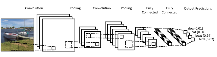
Putting it all together
Convolutional neural networks (also called ConvNets) are typically comprised of convolutional layers with some method of periodic downsampling (either through pooling or strided convolutions). The convolutional layers create feature mappings which serve to explain the input in different ways, while the pooling layers compress the spatial dimensions, reducing the number of parameters needed to extract features in following layers. For image classification, we eventually reduce this representation of our original input into a deep stack of 1 by 1 (single value) representations of the original input. At this time, we can now feed this information into a few fully-connected layers to determine the likelihood of each output class being present in the image.
Further reading
Lectures/notes
- Stanford CS231: Introduction to Convolutional Neural Networks for Visual Recognition
- Deep Learning for Computer Vision (Andrej Karpathy, OpenAI)
- Stanford Stats 385: Theoretical analysis of convnets
Blogs/talks
- François Chollet: Visualizing what convnets learn
- A visual and intuitive understanding of deep learning
- Backpropagation for convolutional neural networks
- Applied Deep Learning - Part 4: Convolutional Neural Networks
- Fifteen questions and answers about the use of convolutional neural networks as a model of the visual system.
- Intuitively Understanding Convolutions for Deep Learning
Papers
- A guide to convolution arithmetic for deep learning
- Visualizing and Understanding Convolutional Networks
- Yann LeCun’s original introduction of CNNs
Demos
- Browser-based convnet with inspectable layers
- Handwritten digits interactive demo and visualization of convolutional neural networks
Visualization tools
-Keras Visualization Toolkit
-Tensorflow Lucid
For a more detailed discussion of the implementations of convolutions, see cuDNN: Efficient Primitives for Deep Learning.