Understanding the attention mechanism in sequence models

In this blog post, we'll discuss a key innovation in sequence-to-sequence model architectures: the attention mechanism. This architecture innovation dramatically improved model performance for sequence-to-sequence tasks such as machine translation and text summarization.
Moreover, the success of this attention mechanism led to the seminal paper, "Attention Is All You Need", which introduced the Transformer model architecture. I'll discuss the Transformer model architecture in subsequent posts, but I feel that it's useful to start by building a foundational understanding of the attention mechanism itself (which is the focus of this post). With that said, let's dive right in!
Overview
- A quick refresher: sequence to sequence models
- The context vector bottleneck
- Introducing the attention mechanism
- Training an attention model
- Benefits of attention: shorter path lengths
- Conclusion
- Resources
A quick refresher: sequence to sequence models
Let us consider the sequence modeling task where we have a variable-length input sequence and we're expected to predict a variable-length output sequence. A common example of this type of task is machine translation, where the input might be "i love you" (English) and the expected output might be "te amo" (Spanish).
Notice how the input length (3 words) doesn't necessarily match the output length (2 words). This poses a challenging sequence prediction task since we can't simply train a model which learns to map each input token to its corresponding output token; there isn't a 1:1 mapping!
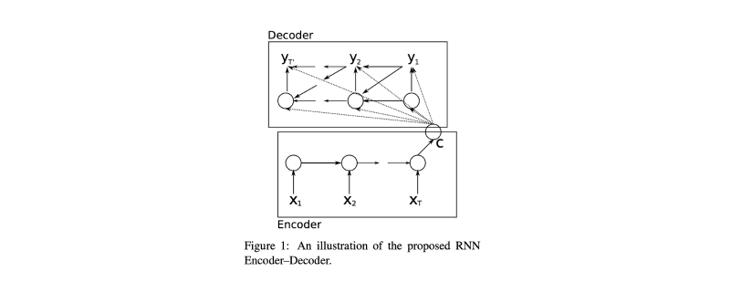
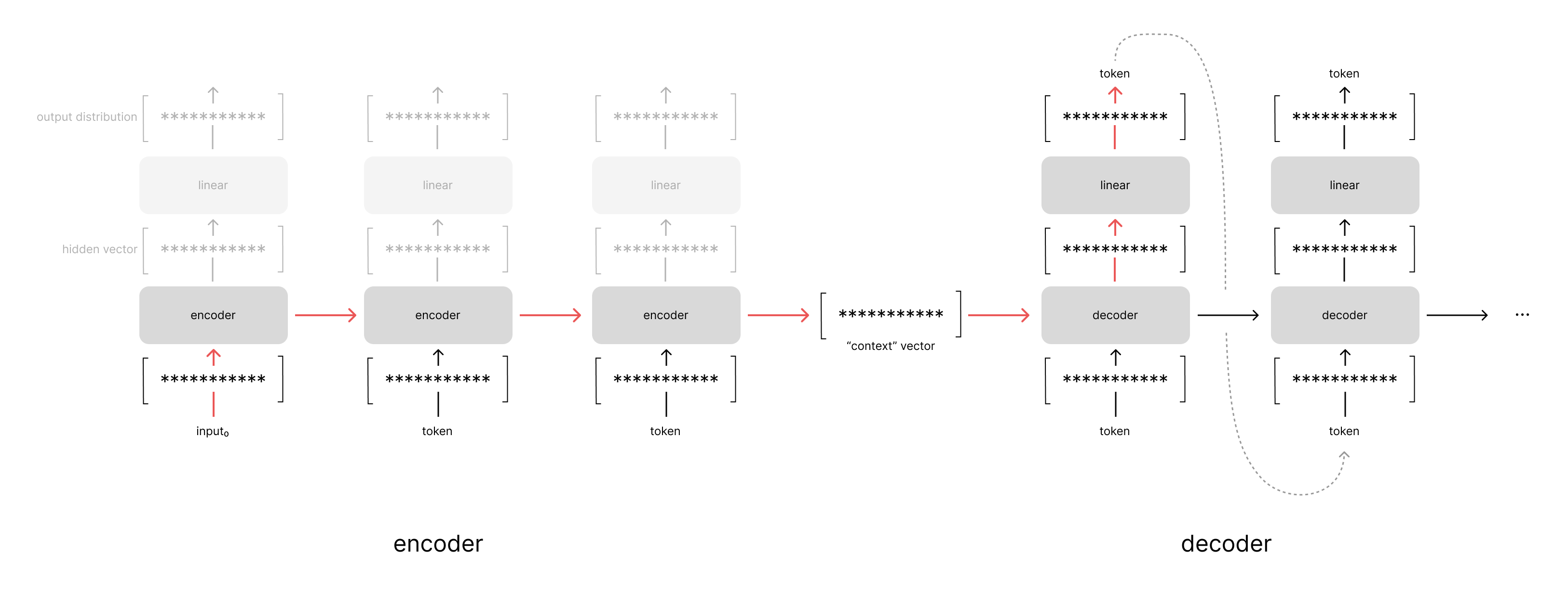
Cho et al introduced the RNN Encoder–Decoder neural network architecture for this type of sequence modeling where the variable-length input is encoded into a fixed-size vector (using a recurrent neural network) which is subsequently decoded into another variable-length output sequence (using a second recurrent neural network).
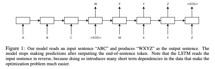
Sutskever et al introduced a similar architecture that builds on this approach using LSTM networks to encode and decode variable-length sequences. In this architecture, however, we simply take the last hidden state of the encoder and use that to initialize the decoder rather than passing it as context to every step during decoding. Also note how the input sequence is reversed in order to make the optimization problem easier, we'll dig deeper into this architecture choice in a later section.
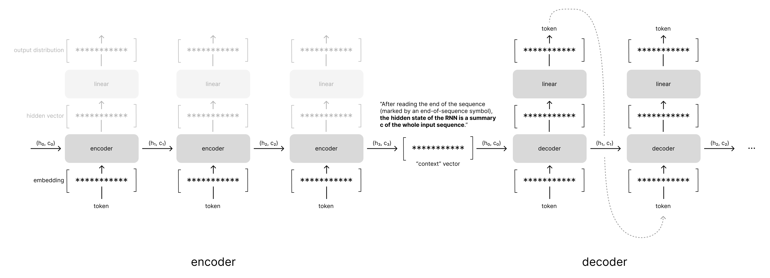
While these two architectures had some slight differences, the overall approach was the same. We encode our variable-length input sequence into a fixed-size vector which provides a summary of the entire input sequence. This summary is then provided as context to the decoder when generating the output sequence.
The context vector bottleneck
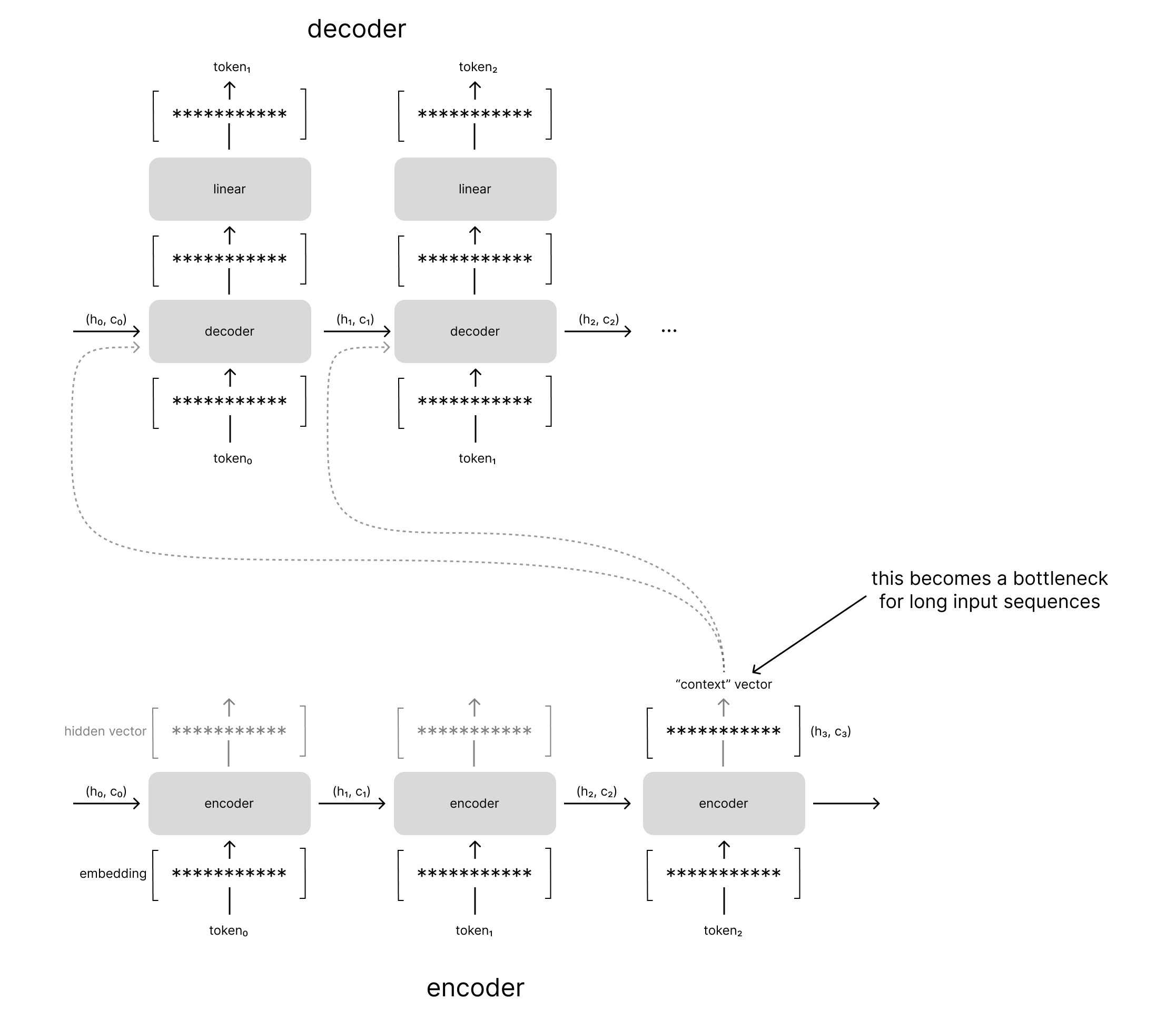
Although the fixed-size context vector enables us to flexibly learn sequence-to-sequence tasks such as machine translation or text summarization, let's consider the implications of this architecture design.
A fixed-size vector implies that there's a fixed amount of information that we can store in our summary of the input sequence. For the sake of an example, let's assume that our context vector can store 100 bits of information. Let's also assume that each time-step in the input sequence contributes equally to the information stored in the context vector. For an input sequence of 5 tokens, each token would contribute 20 bits of information to the context vector. However, for an input sequence of 10 tokens, each token would only contribute 10 bits of information to the context vector.
Through this example one can see how performance may degrade in sequence-to-sequence models for longer input sequences. As the size of the input grows, we can store less and less information per token in the input sequence.
Introducing the attention mechanism
In order to address this context bottleneck challenge, Bahdanau et al introduced a neural network architecture which allows us to build a unique context vector for every decoder time-step based on different weighted aggregations across all of the encoder hidden states.
Whereas in the previous hypothetical example we only had 100 bits of information to summarize the entire input sequence, with this new approach we can provide a hypothetical 100 bits of information about the input sequence at each step of the decoder model.
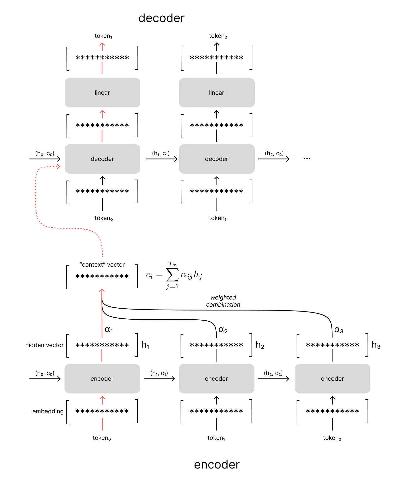
In the example visualized below, you can see how we take a weighted combination across all of the encoder hidden states to produce our context vector, rather than simply using the final hidden state. These weights are determined by an attention mechanism which determines the encoder hidden states that are relevant given the current decoder hidden state. We'll discuss more about how this attention mechanism is trained in the next section.
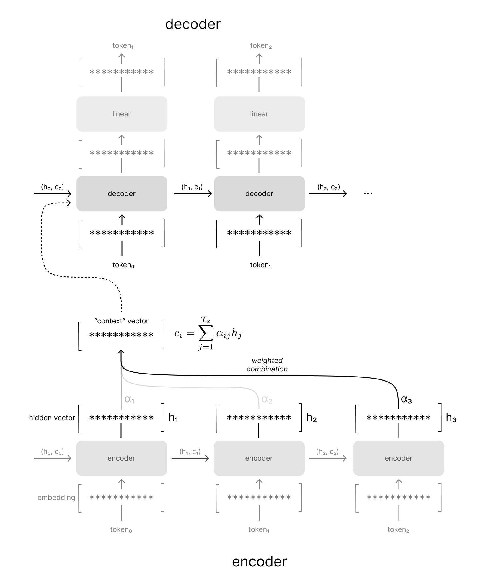
Notice how the attention weights in the example above place most of the weight on the last token of the input sequence when generating the first token of the output sequence. If you recall our running example of translating "i love you" to Spanish, we're effectively aligning the related tokens of "i love you" and "te amo". Bahdanau et al refer to this attention mechanism as an alignment model since it allows the decoder to search across the input sequence for the most relevant time-steps regardless of the temporal position of the decoder model.
When decoding the second token, you can see that we have an entirely different weighted combination of contexts from the encoder hidden states, which helps align the "i love you" with "te amo" (in case you don't speak Spanish, "amo" is the first person singular conjugation of the Spanish word for love).
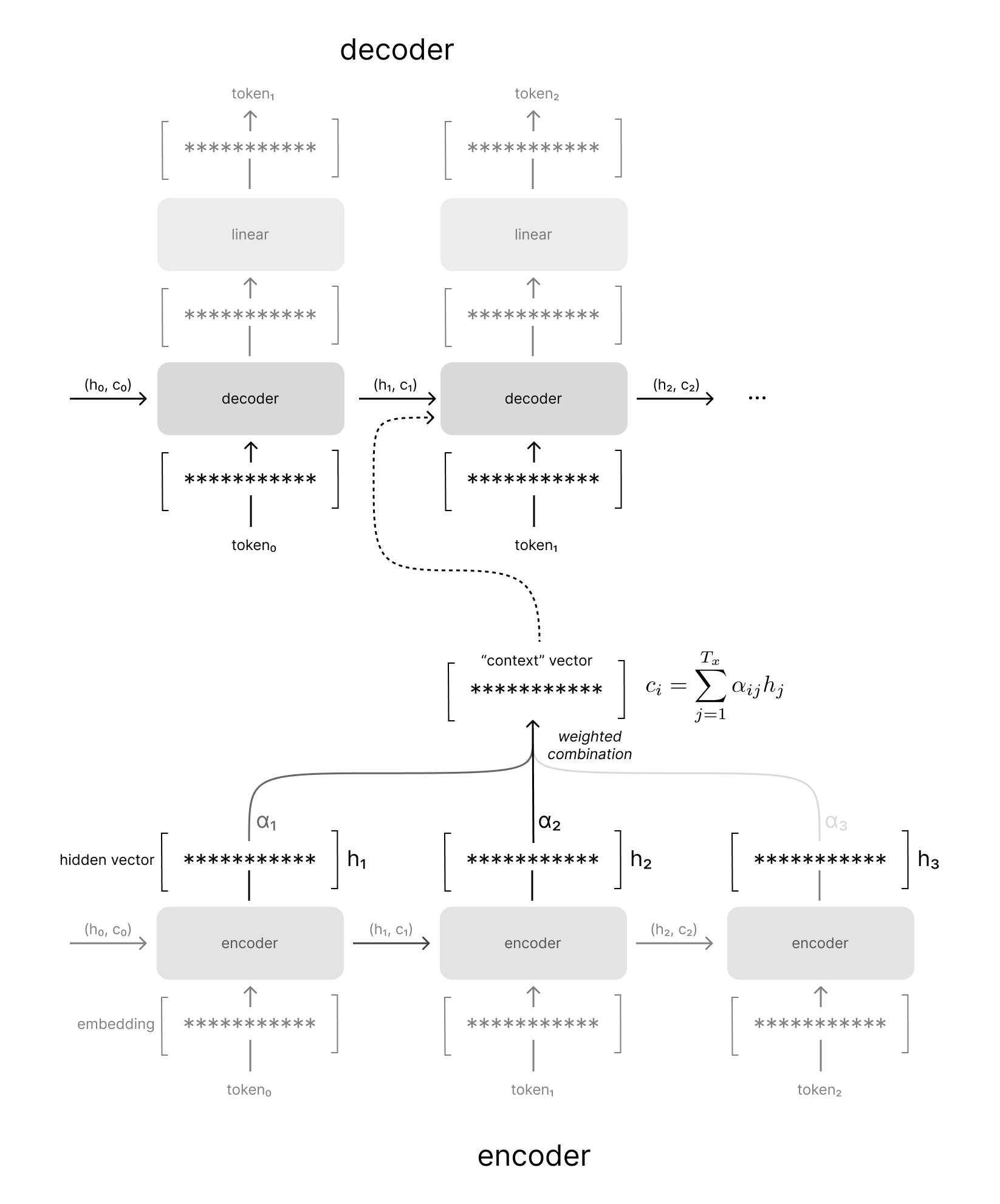
As the decoder model continues to generate the output sequence, we'll continue to compare the current decoder hidden state against all of our encoder hidden states to produce a unique context vector.
Training an attention model
Now that you understand how the attention weights are used to produce a unique context vector at each step in the decoder model, let's dive into the architecture and training process for our attention mechanism.
As we discussed previously, the attention model is effectively comparing a given decoder hidden state with a specific encoder hidden state to determine the relevance between these two vectors.
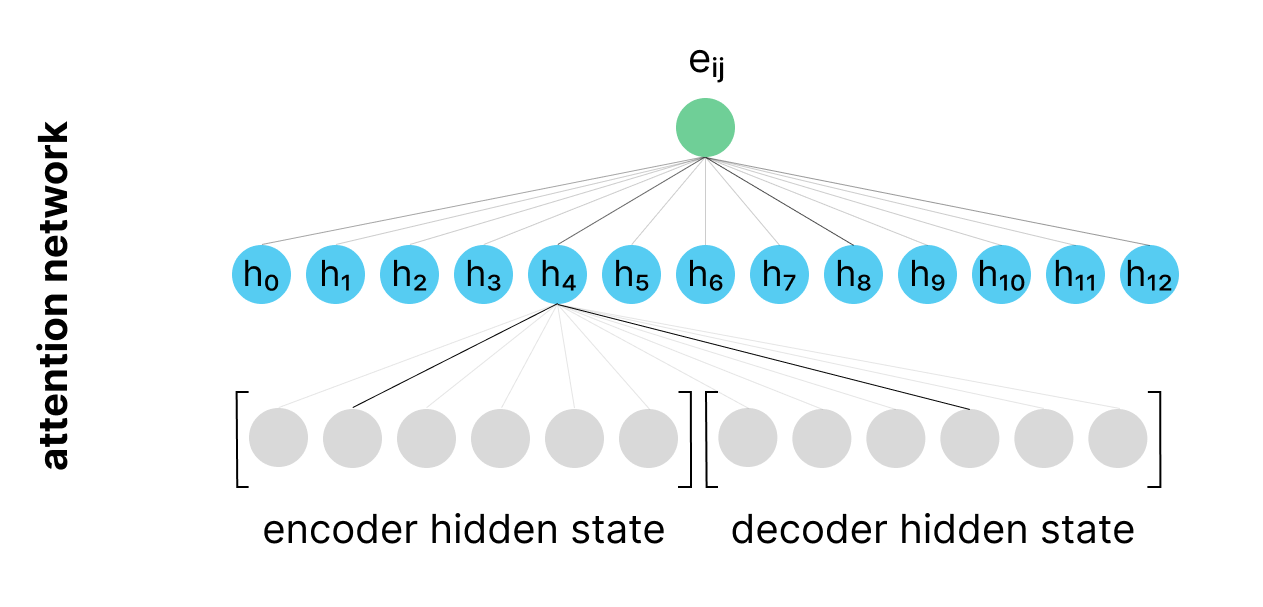
One way to compute this relevance score is to concatenate the encoder hidden state and decoder hidden state vectors and pass them through a multi-layer perception. The hidden layer of our MLP model can learn to identify relationships between certain dimensions in the encoder hidden state and the decoder hidden state. The output of this model is effectively answering the question: "how relevant is the information in this encoder hidden state for computing the next output in the sequence, given my current decoder hidden state?"
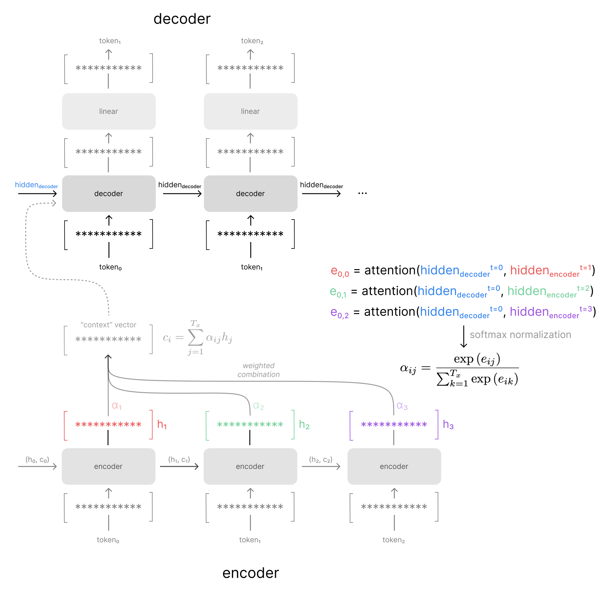
As a concrete example, the figure below visualizes how the attention weights are computed for the first time-step in the decoder model. Notice how we compare the previous decoder hidden state to every encoder hidden state in our sequence. The attention model outputs a "relevance" score (ei,j) for each combination, which we can normalize via the softmax function to obtain our attention weights (αi,j).
This attention mechanism is trained jointly with the rest of the sequence-to-sequence network, since we can backpropagate through the entire calculation of our attention weights and corresponding context vector. This means that the attention model is optimized to find relevant hidden states for the specific sequence-to-sequence task at hand. In other words, the attention mechanism for a machine translation model might learn to find different patterns than the attention mechanism for a text summarization model, depending on what's most useful for the task at hand.
Benefits of attention: shorter path lengths
In a previous section we touched on Sutskever et al's architecture decision to reverse the input sequence in order to make the optimization problem easier. In fact, they state "the simple trick of reversing the words in the source sentence is one of the key technical contributions of this work." Let's dig in to why this may be the case.
Let us assume that, on average, the position of a token in the input sequence is roughly equivalent to its relevant position in the output sequence. For example, in the English to Spanish translation of "this is an example" to "esto es un ejemplo", the first word "this" of the input sequence can be translated directly to the first word "esto" of the output sequence.
Recall that a standard encoder-decoder model architecture (without attention) uses the last hidden state of the encoder model as the context vector. This means that the information from the first time-step of the input sequence must be preserved in the hidden state passed through all of the time-steps in the input sequence. This information is then used to decode the first time-step of the output sequence.
If we instead reverse the order of the input sequence, the information from the first time-step in the input has a shorter path length through the unrolled recurrent networks to the corresponding output. In general, shorter path lengths are desired because it's easier for gradient signals to propagate. Neural networks have historically struggled with learning longer-term dependencies (read: patterns across longer path lengths) due to the vanishing/exploding gradient problem coupled with the fact that we can only store a limited amount of information in our hidden state.
In section 3.3 the authors state:
By reversing the words in the source sentence, the average distance between corresponding words in the source and target language is unchanged. However, the first few words in the source language are now very close to the first few words in the target language, so the problem’s minimal time lag is greatly reduced. Thus, backpropagation has an easier time “establishing communication” between the source sentence and the target sentence, which in turn results in substantially improved overall performance. – Sequence to Sequence Learning with Neural Networks
The trick of reversing the input sequence is effectively making it easier to pass information from the earlier parts of the input sequence while making it harder to pass information from the later parts of the input sequence.
As a quick aside, this tradeoff makes sense when you consider the fact that our decoder model autoregressively generates the output vector. By making it easier for the model to start off with good initial output sequence predictions (by decreasing the path length to the initial input tokens), we're reducing the likelihood of introducing errors early on which would continue to accumulate as you generate the rest of the output sequence.
While this does appear to make the optimization problem easier, reversing the input sequence doesn't have an effect on the average distance between related tokens in the input and output sequences.
Let's contrast this with an encoder-decoder model architecture which leverages attention, where every time-step in the input sequence now has an equal path length to each time-step in the output sequence.
Notice how the information from the encoder's first hidden state is directly available to the decoder; our encoder model no longer needs to remember all of the details from this first time step throughout the entire input sequence.
Because the attention mechanism introduces shorter path lengths at every time step in the input sequence, we no longer need to make a tradeoff regarding which portions of the input sequence are most important for the decoder; the entire sequence is now easier to optimize as a result of shorter path lengths.
Conclusion
Standard encoder-decoder sequence models struggle from an information bottleneck passing information from the encoder to the decoder. The attention mechanism helps alleviate this bottleneck by allowing the decoder to search across the entire input sequence for information at each step during the output sequence generation.
This is accomplished by introducing a small attention model which learns to compute a relevance score between an encoder hidden state and a decoder hidden state. From these relevance scores, we can produce a unique weighted combination of encoder hidden states as context for each step of the decoder model.
Resources
Papers
- Learning Phrase Representations using RNN Encoder-Decoder for Statistical Machine Translation
- Sequence to Sequence Learning with Neural Networks
- Neural Machine Translation by Jointly Learning to Align and Translate
Lectures
Blog posts