Scaling nearest neighbors search with approximate methods.
In this blog post, I'll cover a couple of techniques used for approximate nearest neighbors search. This post will not cover approximate nearest neighbors methods exhaustively, but hopefully you'll be able to understand how people generally approach this problem and how to apply these techniques

Jump to:
What is nearest neighbors search?
In the world of deep learning, we often use neural networks to learn representations of objects as vectors. We can then use these vector representations for a myriad of useful tasks.
To give a concrete example, let's consider the case of a facial recognition system powered by deep learning. For this use case, the objects are images of people's faces and the task is to identify whether or not the person in a submitted photo matches a person in a database of known identities. We'll use a neural network to build vector representations of all of the images; then, performing facial recognition is as simple as taking the vector representation of a submitted image (the query vector) and searching for similar vectors in our database. Here, we define similarity as vectors which are close together in vector-space. (How we actually train a network to produce these vector representations is outside of the scope of this blog post.)
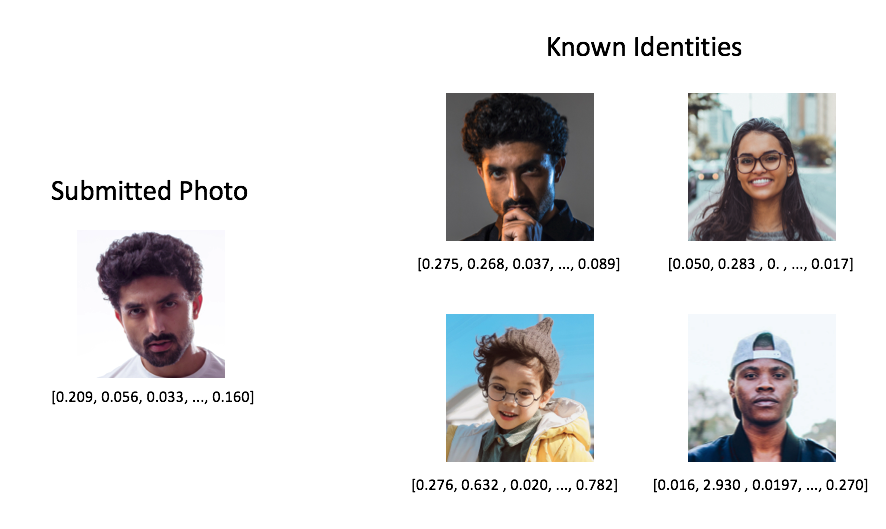
All of these vectors were extracted from a ResNet50 model. Notice how the values in the query vector are quite similar to the vector in the top left of known identities.
The process of finding vectors that are close to our query is known as nearest neighbors search. A naive implementation of nearest neighbors search is to simply calculate the distance between the query vector and every vector in our collection (commonly referred to as the reference set). However, calculating these distances in a brute force manner quickly becomes infeasible as your reference set grows to millions of objects.
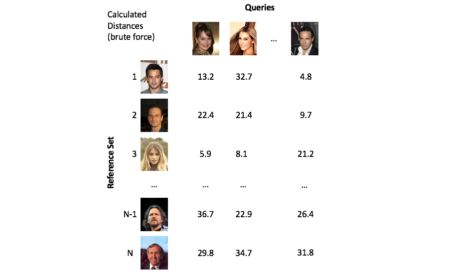
Imagine if Facebook had to compare each face in a new photo against all of its users every time it suggested who to tag, this would be computationally infeasible!
A class of methods known as approximate nearest neighbors search offer a solution to our scaling dilemma by partitioning the vector space in a clever way such that we only need to examine a small subset of the overall reference set.
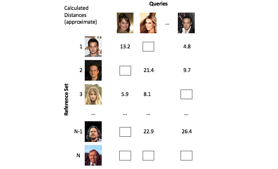
Approximate methods alleviate this computational burden by cleverly partitioning the vectors such that we only need to focus on a small subset of objects.
In this blog post, I'll cover a couple of techniques used for approximate nearest neighbors search. This post will not cover approximate nearest neighbors methods exhaustively, but hopefully you'll be able to understand how people generally approach this problem and how to apply these techniques in your own work.
In general, the approximate nearest neighbor methods can be grouped as:
- Tree-based data structures
- Neighborhood graphs
- Hashing methods
- Quantization
K-dimensional trees
The first approximate nearest neighbors method we'll cover is a tree-based approach. K-dimensional trees generalize the concept of a binary search tree into multiple dimensions.
The general procedure for growing a k-dimensional tree is as follows:
- pick a random dimension from your k-dimensional vector
- find the median of that dimension across all of the vectors in your current collection
- split the vectors on the median value
- repeat!
A toy 2-dimensional example is visualized below. At the top level, we select a random dimension (out of the two possible dimensions, $x_0$ and $x_1$) and calculate the median. Then, we follow the same procedure of picking a dimension and calculating the median for each path independently. This process is repeated until some stopping criterion is satisfied; each leaf node in the tree contains a subset of vectors from our reference set.
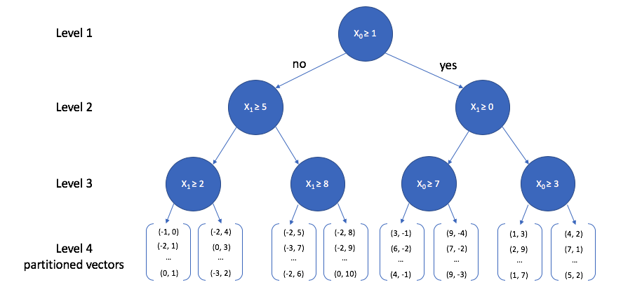
We can view how the two-dimensional vectors are partitioned at each level of the k-d tree in the figure below. Take a minute to verify that this visualization matches what is described in the tree above.
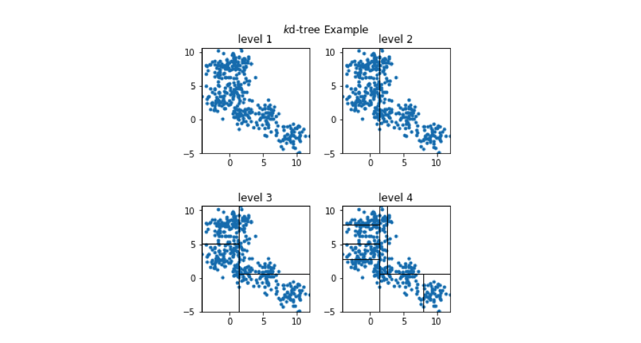
In order to see the usefulness of this tree, let's now consider how we could use this data structure to perform an approximate nearest neighbor query. As we walk down the tree, notice how the highlighted area (the area in vector space that we're interested in) shrinks down to a small subset of the original space. (I'll use the level 4 subplot for this example.)
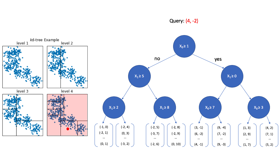
At the top level, we look at the first dimension of the query vector and ask whether or not its value is greater than or equal to 1. Since 4 is greater than 1, we walk down the "yes" path to the next level down. We can safely ignore any of the nodes that follow the first "no" path.
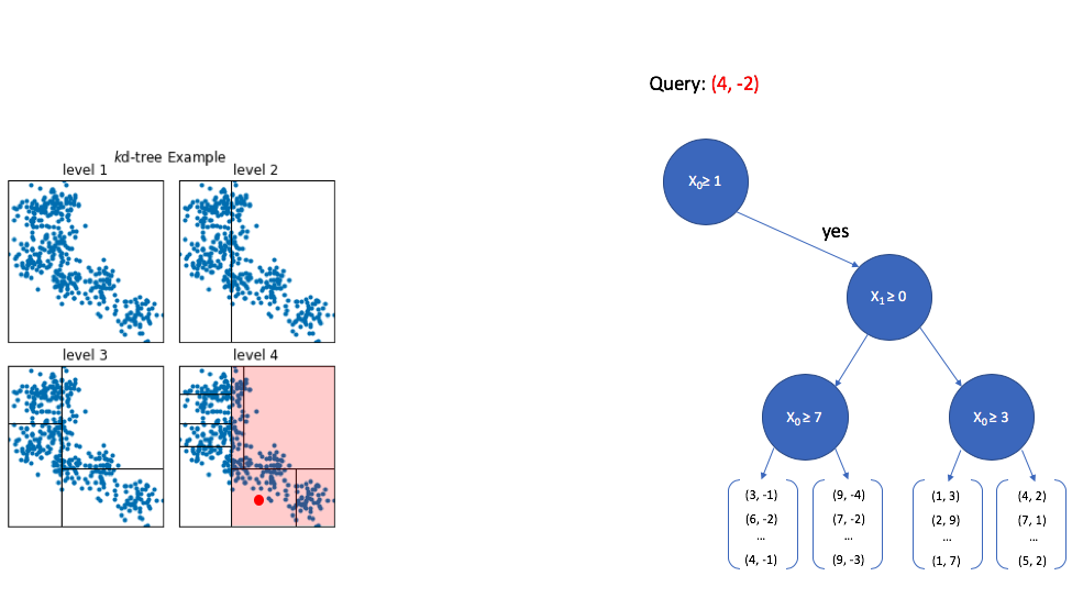
Now we look at the second dimension of the vector and ask whether its value is greater than or equal to 0. Since -2 is less than 0, we now walk down the "no" path. Notice again how the area of interest in our overall vector-space continues to shrink.
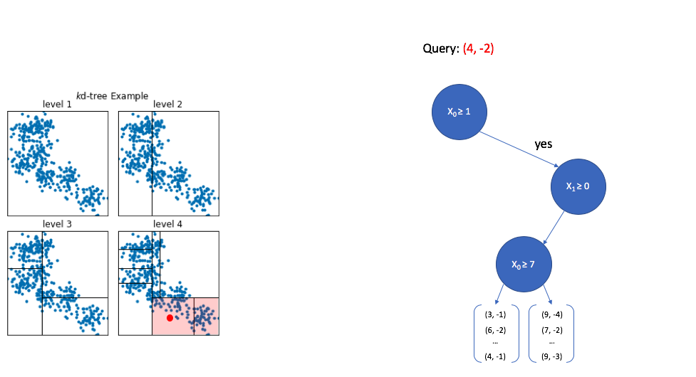
Finally, once we reach the bottom of the tree we are left with a collection of vectors. Thankfully, this is a small subset relative to the overall size of the reference set, so calculating the distance between the query vector and each vector in this subset is computationally feasible.
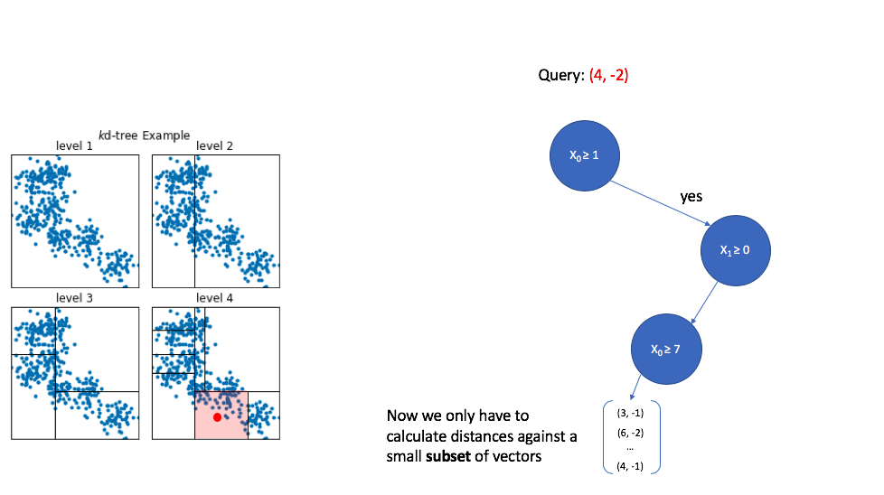
K-d trees are popular due to their simplicity, however, this technique struggles to perform well when dealing with high dimensional data. Further notice how we only returned vectors which are found in the same cell as the query point. In this example, the query vector happened to fall in the middle of a cell, but you could imagine a scenario where the query vector lies near the edge of a cell and we miss out on vectors which lie just outside of the cell.
Quantization
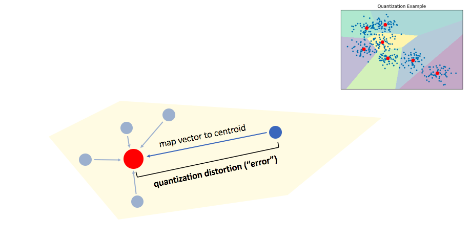
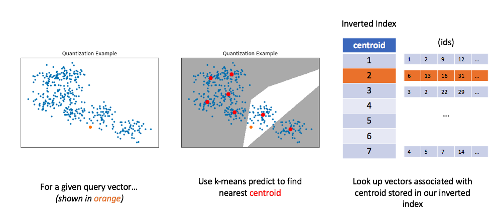
Another approach to the approximate nearest neighbors problem is to collapse our reference set into a smaller collection of representative vectors. We can find these "representative" vectors by simply running the K-means algorithm on our data. In the literature, this collection of "representative" vectors is commonly referred to as the codebook.
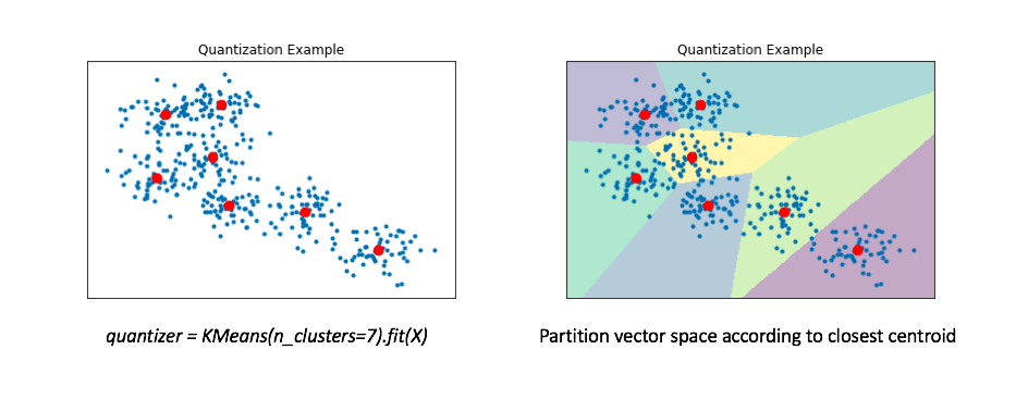
The right figure displays a Voronoi diagram which essentially partitions the space according to the set of points for which a given centroid is closest.
We'll then "map" all of our data onto these centroids. By doing this, we can represent our reference set of a couple hundred vectors with only 7 representative centroids. This greatly reduces the number of distance computations we need to perform (only 7!) when making an nearest neighbors query.
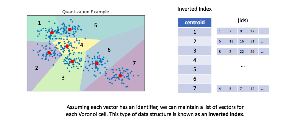
We can then maintain an inverted list to keep track of all of the original objects in relation to which centroid represents the quantized vector.
You can optionally retrieve the full vectors for all of the ids maintained in the inverted list for a given centroid, calculating the true distances between each vector and our query. This is a process known as re-ranking and can improve your query performance.
Similar to before, let's now look at how we can use this method to perform a query. For a given query vector, we'll calculate the distances between the query vector and each centroid in order to find the closest centroid. We can then look up the centroid in our inverted list in order to find all of the nearest vectors.
Unfortunately, in order to get good performance using quantization, you typically need to use very large numbers of centroids for quantization; this impedes on original goal of alleviating the computational burden of calculating too many distances.
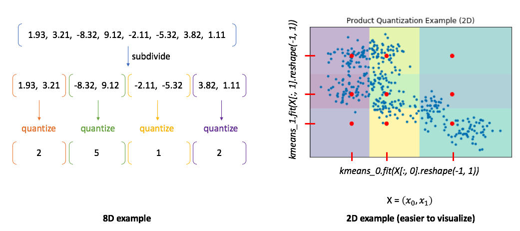
Product quantization
Product quantization addresses this problem by first subdividing the original vectors into subcomponents and then quantizing (ie. running K-means on) each subcomponent separately. A single vector is now represented by a collection of centroids, one for each subcomponent.
To illustrate this, I've provided two examples. In the 8D case, you can see how our vector is divided into subcomponents and each subcomponent is represented by some centroid value. However, the 2D example shows us the benefit of this approach. In this case, we can only split our 2D vector into a maximum of two components. We'll then quantize each dimension separately, squashing all of the data onto the horizontal axis and running k-means and then squashing all of the data onto the vertical axis and running k-means again. We find 3 centroids for each subcomponent with a total of 6 centroids. However, the total set of all possible quantized states for the overall vector is the Cartesian product of the subcomponent centroids.
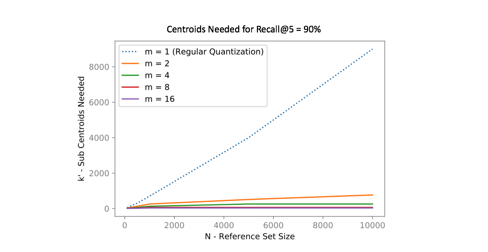
In other words, if we divide our vector into $m$ subcomponents and find $k$ centroids, we can represent $k^m$ possible quantizations using only $km$ vectors! The chart below shows how many centroids are needed in order to get 90% of the top 5 search results correct for an approximate nearest neighbors query. Notice how using product quantization ($m>1$) vastly reduces the number of centroids needed to represent our data. One of the reasons why I love this idea so much is that we've effectively turned the curse of dimensionality into something highly beneficial!
Handling multi-modal data
Product quantization alone works great when our data is distributed relatively evenly across the vector-space. However, in reality our data is usually multi-modal. To handle this, a common technique involves first training a coarse quantizer to roughly "slice" up the vector-space, and then we'll run product quantization on each individual coarse cell.
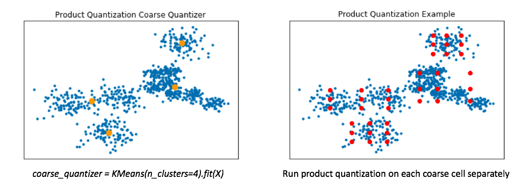
Below, I've visualized the data that falls within a single coarse cell. We'll use product quantization to find a set of centroids which describe this local subset of data, and then repeat for each coarse cell. Commonly, people encode the vector residuals (the difference between the original vector and the closest coarse centroid) since the residuals tend to have smaller magnitudes and thus lead to less lossy compression when running product quantization. In simple terms, we treat each coarse centroid as a local origin and run product quantization on the data with respect to the local origin rather than the global origin.
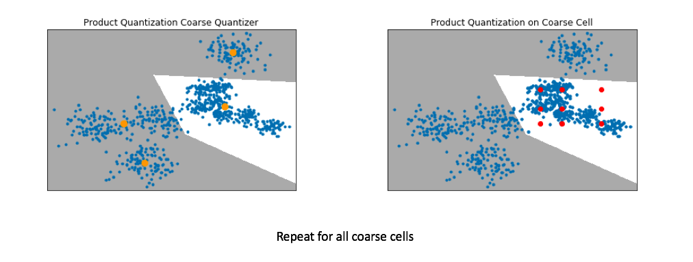
Pro-tip: If you want to scale to really large datasets you can use product quantization as both the coarse quantizer and the fine-grained quantizer within each coarse cell. See this paper for the details.
Locally optimized product quantization
The ideal goal for quantization is to develop a codebook which is (1) concise and (2) highly representative of our data. More specifically, we'd like all of the vectors in our codebook to represent dense regions of our data in vector-space. A centroid in a low-density area of our data is inefficient at representing data and introduces high distortion error for any vectors which fall in its Voronoi cell.
One potential way we can attempt to avoid these inefficient centroids is to add an alignment step to our product quantization. This allows for our product quantizers to better cover the local data for each coarse Voronoi cell.
We can do this by applying a transformation to our data such that we minimize our quantization distortion error. One simple way to minimize this quantization distortion error is to simply apply PCA in order to mean-center the data and rotate it such that the axes capture most of the variance within the data.
Recall my earlier example where we ran product quantization on a toy 2D dataset. In doing so, we effectively squashed all of the data onto the horizontal axis and ran k-means and then repeated this for the vertical axis. By rotating the data such that the axes capture most of the variance, we can more effectively cover our data when using product quantization.
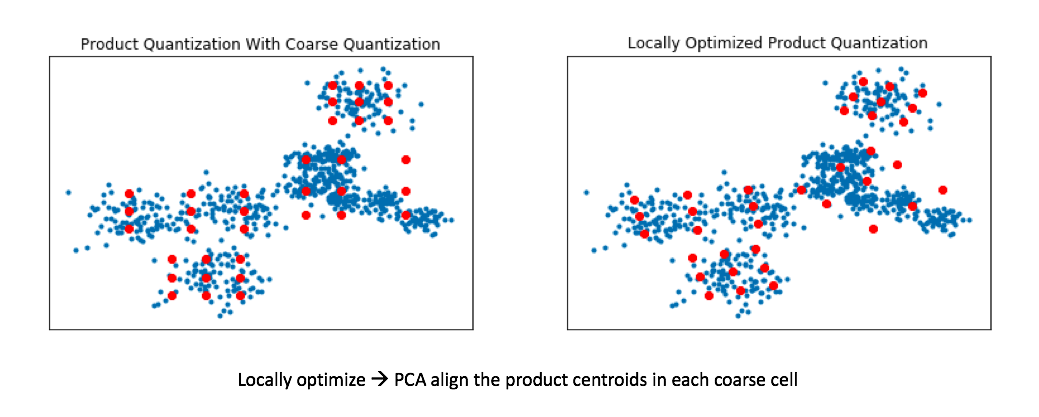
This technique is known as locally optimized product quantization, since we're manipulating the local data within each coarse Voronoi cell in order to optimize the product quantization performance. The authors who introduced this technique have a great illustrative example of how this technique can better fit a given set of vectors.
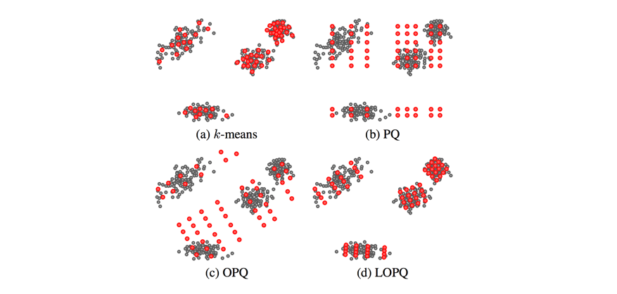
This blog post glances over (c) Optimized Product Quantization which is the same idea of aligning our data for better product quantization performance, but the alignment is performed globally instead of aligning local data in each Voronoi cell independently. Image credit
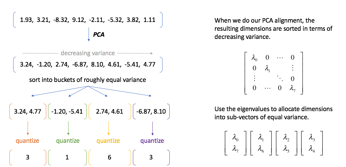
A quick sidenote regarding PCA alignment
The authors who introduced product quantization noted that the technique works best when the vector subcomponents had similar variance. A nice side effect of doing PCA alignment is that during the process we get a matrix of eigenvalues which describe the variance of each principal component. We can use this to our advantage by allocating principal components into buckets of equal variance.
Common datasets
Further reading
Papers
- Product quantization for nearest neighbor search
- Optimized Product Quantization for Approximate Nearest Neighbor Search (see also this presentation)
- Locally Optimized Product Quantization for Approximate Nearest Neighbor Search
- The Inverted Multi-Index
I didn't cover binary codes in this post - but I should have! I may come back and edit the post to include more information soon. Until then, enjoy this paper.
Lectures
Blog posts/talks
- Nearest Neighbor Indexes for Similarity Search
- Scaling Visual Search with Locally Optimized Product Quantization
- Indexing Billions of Text Vectors
- Product Quantizers for k-NN Tutorial Part 1
- Product Quantizers for k-NN Tutorial Part 2
Libraries and Github repos