Grouping data points with k-means clustering.

K-means clustering is a simple method for partitioning $n$ data points in $k$ groups, or clusters.
Essentially, the process goes as follows:
- Select $k$ centroids. These will be the center point for each segment.
- Assign data points to nearest centroid.
- Reassign centroid value to be the calculated mean value for each cluster.
- Reassign data points to nearest centroid.
- Repeat until data points stay in the same cluster.
Here's a nice GIF to visualize the process. The $x$'s are centroids and the colored dots are data points assigned to a cluster.
Image credit
Now let's look at each step in more detail.
Choosing the initial centroid values
Before we discuss how to initialize centroids for k-means clustering, we must first decide how many clusters to partition the data into. As a human, looking at the above example the answer is obviously three. But how could you decide this algorithmically?
Elbow method
One method would be to try many different values of $k$ and plot the average distance of data points from their respective centroid (average within-cluster sum of squares) as a function of $k$. This will give you something along the lines of what is shown below. Notice how increasing the $k$ value from 1 to 2 drastically lowers the average distance of each data point to its respective centroid, but as you continue increasing $k$ the improvements begin to decrease asymptotically. The ideal $k$ value is found at the elbow of such a plot.
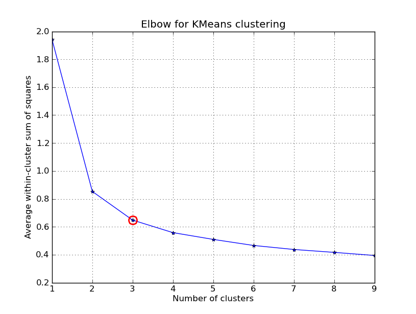
Unfortunately, this isn't exactly an algorithmic approach because it still depends on a manual decision as to where the elbow lies. Further, this method does not always work well when this is no clear distinction of an elbow (for example, when the curve is very smooth).
Silhouette analysis
Another more automated approach would be to build a collection of k-means clustering models with a range of values for $k$ and then evaluate each model to determine the optimal number of clusters.
We can use Silhouette analysis to evaluate each model. A Silhouette coefficient is calculated for observation, which is then averaged to determine the Silhouette score.
The coefficient combines the average within-cluster distance with average nearest-cluster distance to assign a value between -1 and 1. A value below zero denotes that the observation is probably in the wrong cluster and a value closer to 1 denotes that the observation is a great fit for the cluster and clearly separated from other clusters. This coefficient essentially measures how close an observation is to neighboring clusters, where it is desirable to be the maximum distance possible from neighboring clusters.
We can automatically determine the best number of clusters, $k$, by selecting the model which yields the highest Silhouette score.
from sklearn.cluster import KMeans
from sklearn.metrics import silhouette_score
import numpy as np

# Use silhouette score to find optimal number of clusters to segment the data
num_clusters = np.arange(2,10)
results = {}
for size in num_clusters:
    model = KMeans(n_clusters = size).fit(data)
    predictions = model.predict(data)
    results[size] = silhouette_score(data, predictions)

best_size = max(results, key=results.get)
You can also manually inspect the Silhouette coefficients, as discussed in this example.
Centroid initialization
Once you've selected how many groups you'd like to partition your data into, there are a few options for picking initial centroid values. The simplest method? Select $k$ random points from your data set and call it a day. However, it's important to remember that k-means clustering results in an approximate solution converging to a local optimum - so it's possible that starting with a poor selection of centroids could mess up your clustering (ie. selecting an outlier as a centroid). The common solution to this is to run the clustering algorithm multiple times and select the initial values which end up with the best clustering performance (measured by minimum average distance to centroids - typically using within-cluster sum of squares). You can specify the number of random initializations to perform for a K-means clustering model in sci-kit learn using the n_init parameter.
Another method would be to use another clustering technique, such as hierarchical clustering, on a sample of your data set and using the resultant cluster centroids as your initial k-means centroids. This method is typically reserved for k-means clustering applications on large datasets. You could also select your initial values in the most disperse manner possible (maximizing distance between centroids) in order to prevent unwanted localized convergence.
Assigning data points to a cluster
Once you've selected the initial centroids, the next step is to assign each data point to a cluster. Mathematically speaking, you do this:
where clusters are represented as sets $S_{1}$ ,..., $S_{i}$ and the $m$ represents the centroid value (which is a mean in all subsequent steps after the first).
Translating this to English, we get the following:
Set $i$ contains all data points ($x$) in which the distance from the data point ($x_{p}$) to the mean of $i$ ($m_{i}$) is smaller than that of the distance from the data point to the mean of all other centroids ($m_{j}$).
Calculate new centroid values
After each data point is assigned to a cluster, reassign the centroid value for each cluster to be the mean value of all the data points within the cluster.
Reassign data points to new clusters
This is where the iterative process begins. Follow the same process for initially assigning data points to clusters, this time with new centroid values. Iteratively calculate new centroid values and reassign data points until you converge on a cluster segmentation that stops changing.
Dealing with a large data set and don't want to have to perform multiple iterations over your data? Check out the Bradley-Fayyad-Reina algorithm, which performs a similar function as k-means with only one pass through the data.
Example Code
Let's look at an implementation of k-means to group flowers in the Iris data set. First we'll import a few libraries and load the data set.
from sklearn import datasets
from sklearn.cluster import KMeans
from scipy.spatial.distance import cdist, pdist
import numpy as np

iris = datasets.load_iris()
# attributes of iris are ['target_names', 'data', 'target', 'DESCR', 'feature_names']
From this we can see that we'll be clustering the data base on the following features:
- Sepal length (cm)
- Sepal width (cm)
- Petal length (cm)
- Petal width (cm)
Next, we have to choose how many groups we'd like to separate the data into.
# Choosing the optimal k
k_range = range(1,10)
# Try clustering the data for k values ranging 1 to 10
k_means_var = [KMeans(n_clusters = k).fit(iris.data) for k in k_range]
centroids = [X.cluster_centers_ for X in k_means_var]

k_euclid = [cdist(iris.data, cent, 'euclidean') for cent in centroids]
dist = [np.min(ke, axis=1) for ke in k_euclid]

# Calculate within-cluster sum of squares
wcss = [sum(d**2) for d in dist]

# Visualize the elbow method for determining k
import matplotlib.pyplot as plt
plt.plot(k_range, wcss)
plt.show()
Inspecting this plot, k=3 seems like the best choice.
kmeans = KMeans(n_clusters = 3)
kmeans.fit(iris.data)
kmeans.labels_
Let's see how we did. The labels returned by the k-means algorithm are:
>> kmeans.labels_

array([1, 1, 1, 1, 1, 1, 1, 1, 1, 1, 1, 1, 1, 1, 1, 1, 1, 1, 1, 1, 1, 1, 1, 1, 1, 1, 1, 1, 1, 1, 1, 1, 1, 1, 1, 1, 1, 1, 1, 1, 1, 1, 1, 1, 1, 1, 1, 1, 1, 1, 0, 0, 2, 0, 0, 0, 0, 0, 0, 0, 0, 0, 0, 0, 0, 0, 0, 0, 0, 0, 0, 0, 0, 0, 0, 0, 0, 2, 0, 0, 0, 0, 0, 0, 0, 0, 0, 0, 0, 0, 0, 0, 0, 0, 0, 0, 0, 0, 0, 0, 2, 0, 2, 2, 2, 2, 0, 2, 2, 2, 2, 2, 2, 0, 0, 2, 2, 2, 2, 0, 2, 0, 2, 0, 2, 2, 0, 0, 2, 2, 2, 2, 2, 0, 2, 2, 2, 2, 0, 2, 2, 2, 0, 2, 2, 2, 0, 2, 2, 0])
And the labels in the original dataset are:
>> iris.target

array([0, 0, 0, 0, 0, 0, 0, 0, 0, 0, 0, 0, 0, 0, 0, 0, 0, 0, 0, 0, 0, 0, 0, 0, 0, 0, 0, 0, 0, 0, 0, 0, 0, 0, 0, 0, 0, 0, 0, 0, 0, 0, 0, 0, 0, 0, 0, 0, 0, 0, 1, 1, 1, 1, 1, 1, 1, 1, 1, 1, 1, 1, 1, 1, 1, 1, 1, 1, 1, 1, 1, 1, 1, 1, 1, 1, 1, 1, 1, 1, 1, 1, 1, 1, 1, 1, 1, 1, 1, 1, 1, 1, 1, 1, 1, 1, 1, 1, 1, 1, 2, 2, 2, 2, 2, 2, 2, 2, 2, 2, 2, 2, 2, 2, 2, 2, 2, 2, 2, 2, 2, 2, 2, 2, 2, 2, 2, 2, 2, 2, 2, 2, 2, 2, 2, 2, 2, 2, 2, 2, 2, 2, 2, 2, 2, 2, 2, 2, 2, 2])
From this, we can see that our algorithm did a decent job clustering the first and second flower type, but it sometimes confused the third flower type for the second. Note that our algorithm was blind to any labels associated with the data; it's just putting the data points into groups. This is why the labels don't match up across our results and the provided labels.
Feel like playing around more with k-means clustering? Check out this interactive demonstration.