Evaluating a machine learning model.

So you've built a machine learning model and trained it on some data... now what? In this post, I'll discuss how to evaluate your model, and practical advice for improving the model based on what we learn evaluating it.
I'll answer questions like:
- How well is my model doing? Is it a useful model?
- Will training my model on more data improve its performance?
- Do I need to include more features?
The train/test/validation split
The most important thing you can do to properly evaluate your model is to not train the model on the entire dataset. I repeat: do not train the model on the entire dataset. I talked about this in my post on preparing data for a machine learning model and I'll mention it again now because it's that important. A typical train/test split would be to use 70% of the data for training and 30% of the data for testing.
As I discussed previously, it's important to use new data when evaluating our model to prevent the likelihood of overfitting to the training set. However, sometimes it's useful to evaluate our model as we're building it to find that best parameters of a model - but we can't use the test set for this evaluation or else we'll end up selecting the parameters that perform best on the test data but maybe not the parameters that generalize best. To evaluate the model while still building and tuning the model, we create a third subset of the data known as the validation set. A typical train/test/validation split would be to use 60% of the data for training, 20% of the data for validation, and 20% of the data for testing.
I'll also note that it's very important to shuffle the data before making these splits so that each split has an accurate representation of the dataset.
Metrics
In this session, I'll discuss common metrics used to evaluate models.
Classification metrics
When performing classification predictions, there's four types of outcomes that could occur.
- True positives are when you predict an observation belongs to a class and it actually does belong to that class.
- True negatives are when you predict an observation does not belong to a class and it actually does not belong to that class.
- False positives occur when you predict an observation belongs to a class when in reality it does not.
- False negatives occur when you predict an observation does not belong to a class when in fact it does.
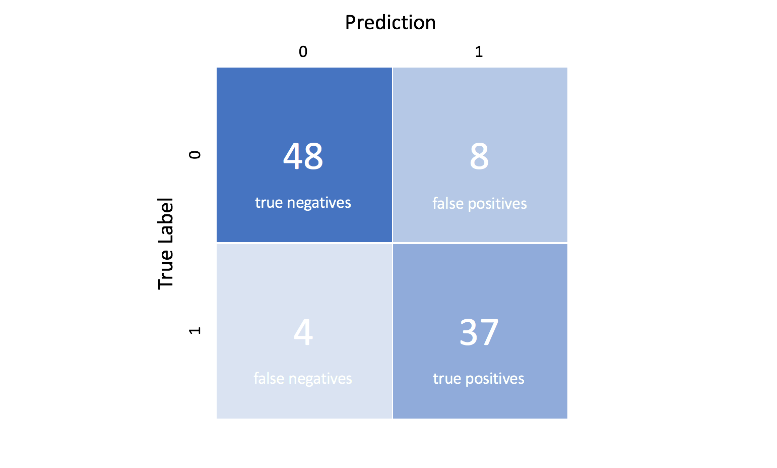
These four outcomes are often plotted on a confusion matrix. The following confusion matrix is an example for the case of binary classification. You would generate this matrix after making predictions on your test data and then identifying each prediction as one of the four possible outcomes described above.
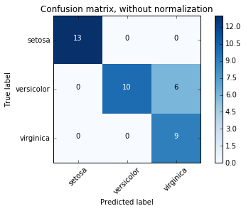
You can also extend this confusion matrix to plot multi-class classification predictions. The following is an example confusion matrix for classifying observations from the Iris flower dataset.
The three main metrics used to evaluate a classification model are accuracy, precision, and recall.
Accuracy is defined as the percentage of correct predictions for the test data. It can be calculated easily by dividing the number of correct predictions by the number of total predictions.
[{\rm{accuracy = }}\frac{{{\rm{correct \hspace{2mm} predictions}}}}{{{\rm{all \hspace{2mm} predictions}}}}]
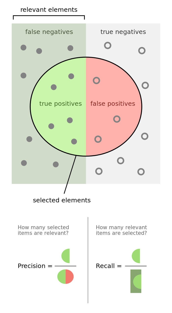
Precision is defined as the fraction of relevant examples (true positives) among all of the examples which were predicted to belong in a certain class.
[{\rm{precision}} = \frac{{{\rm{true \hspace{2mm} positives}}}}{{{\rm{true \hspace{2mm} positives + false \hspace{2mm} positives}}}}]
Recall is defined as the fraction of examples which were predicted to belong to a class with respect to all of the examples that truly belong in the class.
[{\rm{recall}} = {\rm{ }}\frac{{{\rm{true \hspace{2mm} positives}}}}{{{\rm{true \hspace{2mm} positives + false \hspace{2mm} negatives}}}}]
The following graphic does a phenomenal job visualizing the difference between precision and recall.
Precision and recall are useful in cases where classes aren't evenly distributed. The common example is for developing a classification algorithm that predicts whether or not someone has a disease. If only a small percentage of the population (let's say 1%) has this disease, we could build a classifier that always predicts that the person does not have the disease, we would have built a model which is 99% accurate and 0% useful.
However, if we measured the recall of this useless predictor, it would be clear that there was something wrong with our model. In this example, recall ensures that we're not overlooking the people who have the disease, while precision ensures that we're not misclassifying too many people as having the disease when they don't. Obviously, you wouldn't want a model that incorrectly predicts a person has cancer (the person would end up in a painful and expensive treatment process for a disease they didn't have) but you also don't want to incorrectly predict a person does not have cancer when in fact they do. Thus, it's important to evaluate both the precision and recall of a model.
Ultimately, it's nice to have one number to evaluate a machine learning model just as you get a single grade on a test in school. Thus, it makes sense to combine the precision and recall metrics; the common approach for combining these metrics is known as the f-score.
[{F _\beta } = \left( {1 + {\beta ^2}} \right)\frac{{{\rm{precision}} \cdot {\rm{recall}}}}{{\left( {{\beta ^2} \cdot {\rm{precision}}} \right) + {\rm{recall}}}}]
The $\beta$ parameter allows us to control the tradeoff of importance between precision and recall. $\beta < 1$ focuses more on precision while $\beta > 1$ focuses more on recall.
When I was searching for other examples to explain the tradeoff between precision and recall, I came across the following article discussing using machine learning to predict suicide. In this case, we'd want to put much more focus on the model's recall than its precision. It would be much less harmful to have an intervention with someone who was not actually considering suicide than it would be to miss someone who was considering suicide. However, precision is still important because you don't want too many instances where your model predicts false positives or else you have the case of "The Model Who Cried Wolf" (this is the reference for those not familiar with the story).
Note: The article only reports the accuracy of these models, not the precision or recall! By now you should know that accuracy alone is not too informative regarding a model's effectiveness. The original paper published, however, does present the precision and recall.
Regression metrics
Evaluation metrics for regression models are quite different than the above metrics we discussed for classification models because we are now predicting in a continuous range instead of a discrete number of classes. If your regression model predicts the price of a house to be $400K and it sells for $405K, that's a pretty good prediction. However, in the classification examples we were only concerned with whether or not a prediction was correct or incorrect, there was no ability to say a prediction was "pretty good". Thus, we have a different set of evaluation metrics for regression models.
Explained variance compares the variance within the expected outcomes, and compares that to the variance in the error of our model. This metric essentially represents the amount of variation in the original dataset that our model is able to explain.
$$ EV\left( {{y_{true}},{y_{pred}}} \right) = 1 - \frac{{Var\left( {{y_{true}} - {y_{pred}}} \right)}}{{{y_{true}}}} $$
Mean squared error is simply defined as the average of squared differences between the predicted output and the true output. Squared error is commonly used because it is agnostic to whether the prediction was too high or too low, it just reports that the prediction was incorrect.
[{\rm{MSE}}\left( {{y _{true}},{y _{pred}}} \right) = \frac{1}{{{n _{samples}}}}{\sum {\left( {{y _{true}} - {y _{pred}}} \right)} ^2}]
The R2 coefficient represents the proportion of variance in the outcome that our model is capable of predicting based on its features.
[{R^2}\left( {{y _{true}},{y _{pred}}} \right) = 1 - \frac{{{{\sum {\left( {{y _{true}} - {y _{pred}}} \right)} }^2}}}{{{{\sum {\left( {{y _{true}} - \bar y} \right)} }^2}}}]
[\bar y = \frac{1}{{{n _{samples}}}}\sum {{y _{true}}} ]
Bias vs Variance
The ultimate goal of any machine learning model is to learn from examples and generalize some degree of knowledge regarding the task we're training it to perform. Some machine learning models provide the framework for generalization by suggesting the underlying structure of that knowledge. For example, a linear regression model imposes a framework to learn linear relationships between the information we feed it. However, sometimes we provide a model with too much pre-built structure that we limit the model's ability to learn from the examples - such as the case where we train a linear model on a exponential dataset. In this case, our model is biased by the pre-imposed structure and relationships.
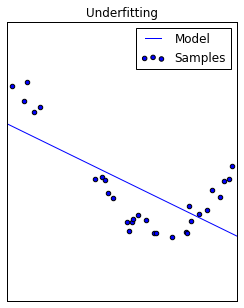
Models with high bias pay little attention to the data presented; this is also known as underfitting.
It's also possible to bias a model by trying to teach it to perform a task without presenting all of the necessary information. If you know the constraints of the model are not biasing the model's performance yet you're still observed signs of underfitting, it's likely that you are not using enough features to train the model.
On the other extreme, sometimes when we train our model it learns too much from the training data. That is, our model captures the noise in the data in addition to the signal. This can cause wild fluctuations in the model that does not represent the true trend; in this case, we say that the model has high variance. In this case, our model does not generalize well because it pays too much attention to the training data without consideration for generalizing to new data. In other words, we've overfit the model to the training data.
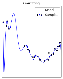
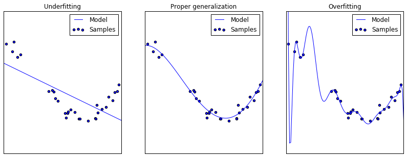
In summary, a model with high bias is limited from learning the true trend and underfits the data. A model with high variance learns too much from the training data and overfits the data. The best model sits somewhere in the middle of the two extremes.
Next, I'll discuss two common tools that are used to diagnosed whether a model is susceptible to high bias or variance.
Validation curves
As we discussed in the previous section, the goal with any machine learning model is generalization. Validation curves allow us to find the sweet spot between underfitting and overfitting a model to build a model that generalizes well.
A typical validation curve is a plot of the model's error as a function of some model hyperparameter which controls the model's tendency to overfit or underfit the data. The parameter you choose depends on the specific model you're evaluating; for example, you might choose to plot the degree of polynomial features (typically, this means you have polynomial features up to this degree) for a linear regression model. Generally, the chosen parameter will have some degree of control over the model's complexity. On this curve, we plot both the training error and the validation error of the model. Using both of these errors combined, we can diagnose whether a model is suffering from high bias or high variance.
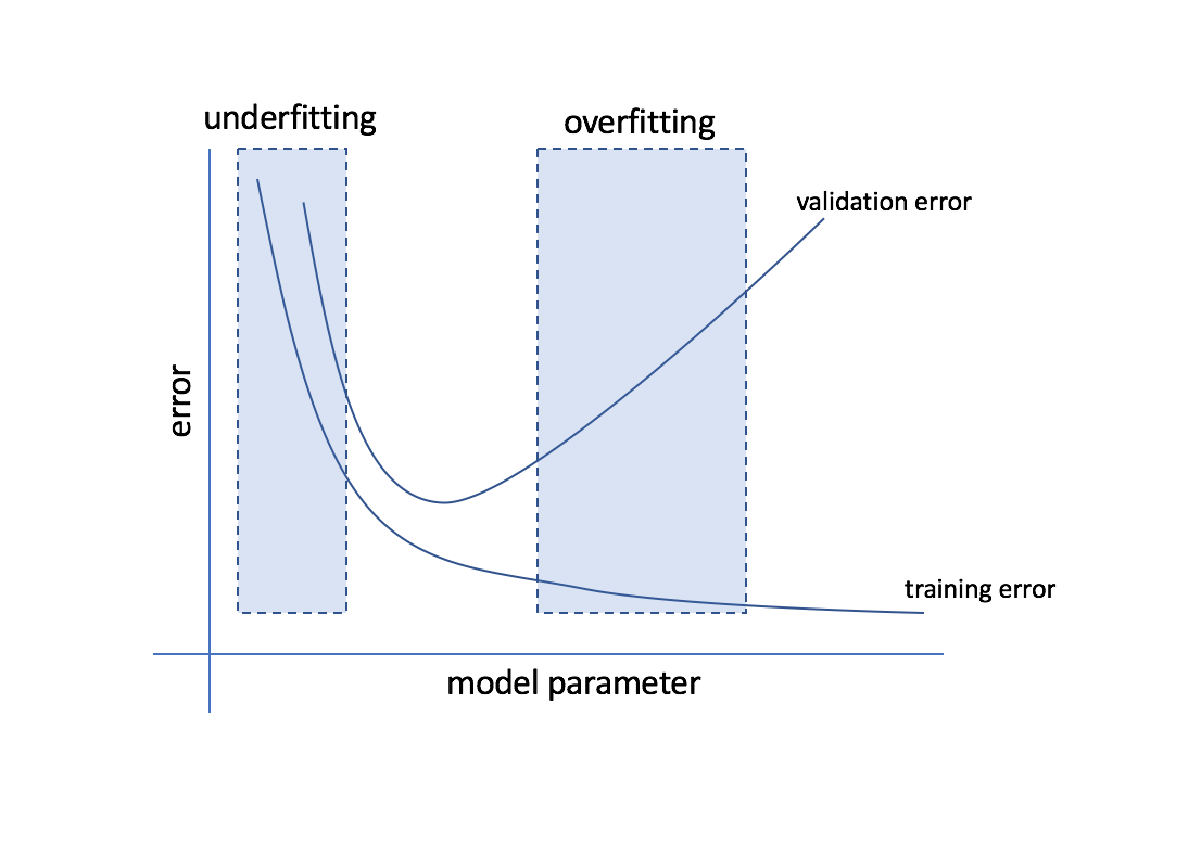
In the region where both the training error and validation error are high, the model is subject to high bias. Here, it was not able to learn from the data and it performing poorly.
In the region where the training error and validation error diverge, with the training error staying low and validation error increasing, we're beginning to see the effects of high variance. The training error is low because we're overfitting the data and learning too much from the training examples, while the validation error remains high because our model isn't able to generalize from the training data to new data.
Learning curves
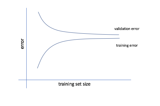
The second tool we'll discuss for diagnosing bias and variance in a model is learning curves. Here, we'll plot the error of a model as a function of the number of training examples. Similar to validation curves, we'll plot the error for both the training data and validation data.
If our model has high bias, we'll observe fairly quick convergence to a high error for the validation and training datasets. If the model suffers from high bias, training on more data will do very little to improve the model. This is because models which underfit the data pay little attention to the data, so feeding in more data will be useless. A better approach to improving models which suffer from high bias is to consider adding additional features to the dataset so that the model can be more equipped to learn the proper relationships.
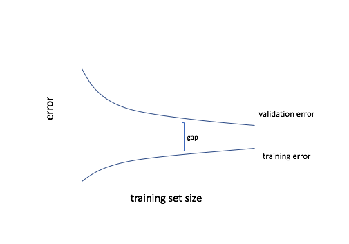
If our model has high variance, we'll see a gap between the training and validation error. This is because the model is performing well for the training data, since it has been overfit to that subset, and performs poorly for the validation data since it was not able to generalize the proper relationships. In this case, feeding more data during training can help improve the model's performance.
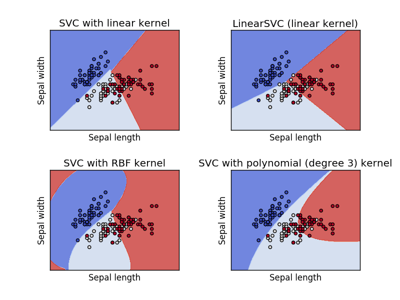
Other practical advice
Another common thing I'll do when evaluating classifier models is to reduce the dataset into two dimensions and then plot the observations and decision boundary. Sometimes it's helpful to visually inspect the data and your model when evaluating its performance.