Planning in a stochastic environment.

In this post, I'll be discussing how to calculate the best set of actions to complete a task whilst operating in a known environment, otherwise known as planning. For this scenario, we have complete knowledge over the system's dynamics including the reward of each state and a probabilistic model for how the agent changes its state. This post will establish the groundwork for eventually discussing reinforcement learning, where our agent doesn't have access to the underlying system dynamics.
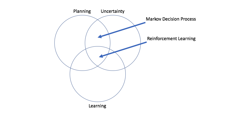
Markov Decision Process
The Markov Decision Process is a method for planning in a stochastic environment. Whereas we cannot control or optimize the randomness that occurs, we can optimize our actions within a random environment. Planning for stochastic environments is much more difficult than planning for a deterministic environment; given the randomness present, there's a degree of uncertainty surrounding the results of our actions.
Specifically, planning refers to figuring out a set of actions to complete a given task. The Markov Decision Process is useful framework for directly solving for the best set of actions to take in a random environment.
An environment used for the Markov Decision Process is defined by the following components:
- An agent is the object within the environment who is encouraged to complete a given task.
- The agent assumes a state within the environment and can traverse the environment by changing its state.
- The agent can change its state by performing an action from a defined set of possible actions.
- A transfer function defines how the agent enters its new state after completing an action. This transfer function is a probabilistic distribution of potential states, introducing stochastic behavior into the environment. Further, this transfer function only depends on the current state - it does not require the entire history of previous actions. This upholds what is known as the Markov property.
- A reward function serves to encourage the agent to complete the given task.
Given this environment, we can develop a policy which describes the best action to take for any given state in the environment. As an agent traverses its environment, it will refer to the policy in order to perform the next action.
A simple example
To provide a concrete example of the defined environment above, take a look a the following image.
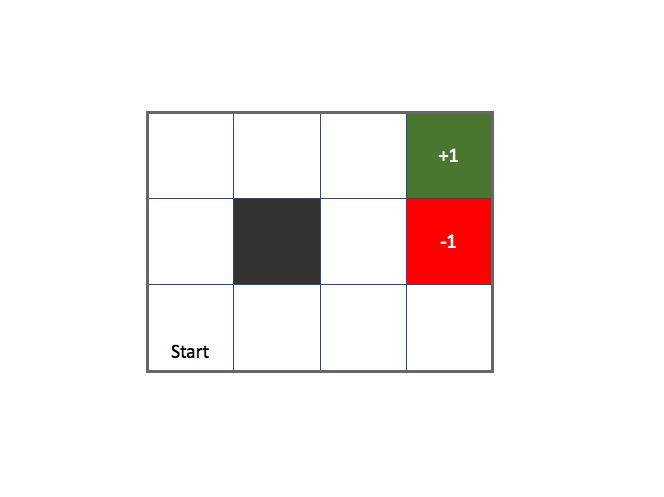
Each square in this figure represents a possible state (excluding the black square, let's say this is an infinitely high barrier). An agent starts at the bottom left and can move from state to state with the following set of actions: up, down, left, right. If the agent is at one of the squares on the perimeter of the environment and tries to take a step outside of the environment, it simply runs into a wall and stays in its current state. The top right square is the desired end state, rewarding the agent with a score of +1 and ending the "game". The square right below it also ends the "game", but rewards the agent with a penalty of -1.
Introducing stochastic behavior to the environment
Now let's define our transfer function. In a deterministic world, if the agent was instructed (by the policy) to move "up" it would do just that. However, suppose your agent is an angsty teenager and only listens to instructions 80% of the time. 10% of the time, the agent moves 90 degrees to the left of the instructed action and 10% of the time the agent moves 90 degrees to the right of the instructed action.
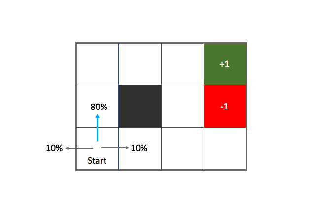
Here, the blue arrow represents the instructed action whereas all of the arrows represent possible outcomes. This introduces a degree of uncertainty, which is useful for more than just modeling angsty teenagers. For example, if you're relying on sensor data to provide information for an autonomous robot, you need to take the noise from a sensor into account when using that information. Modeling stochastic behavior allows us to build more dependable (robust) systems by understanding the undependable nature of our information.
Now that we've introduced stochastic behavior, note how your optimal set of actions will change. Originally, the shortest sequence from start to finish in this environment was either {up, up, right, right, right} or {right, right, up, up, right}. However, now that we've introduced the transfer function where our agent only performs the expected action 80% of the time, the former route seems like a "safer" route than the latter because it is less likely that we'll end up accidentally entering the red state.
Defining rewards
The reward function largely controls the behavior of our agent. This function maps a reward to every state in the environment; thus, for the above example we'll have a reward for the white states in addition to the predefined reward for the green and red states.
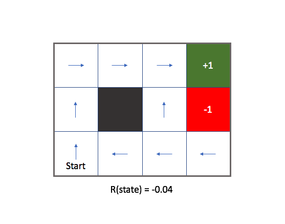
If we'd like to encourage the agent to reach the green state in the shortest amount of time possible, we can assign a small penalty (negative reward) for the remaining states. The following image displays the optimal policy (denoted by blue arrows) for an environment where each white state has a reward of -0.04.
At the risk of introducing redundant terminology in the field, I'll make a distinction between the two types of rewards we've seen thus far.
- Objective state rewards drive the end behavior of our agent to complete a given task. In our example, this is 1) go to the green square and 2) avoid the red square.
- Latent state rewards define how the agent operates in the environment on its journey to achieve the objective rewards. This is the reward given for each white state in our example to encourage our agent to reach the end state quickly.
We can observe the effect of our reward function on the optimal policy by changing the latent state reward value.
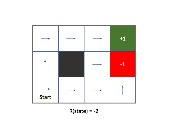
If we make each state have a latent reward that is too large of penalty (in order to encourage the agent to end the game), our agent isn't so careful to avoid the red state. The penalty for existing is harsher than that of entering the red state, so our agent becomes suicidal.
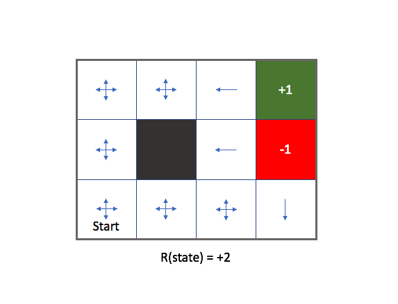
If we make each state have a positive latent reward, the agent has no incentive to ever end the game and aimlessly wanders through the environment collecting the latent reward at each of the white states. In this event, our agent becomes a hedonist and doesn't care about accomplishing the goal.
Thus, finding the right reward function is critical to properly encourage your agent to complete a task.
Utility of a state
One could intuit that it might be helpful to be able to calculate the usefulness of a sequence of states, such that our "view of the future" isn't limited to our direct next action. For example, rather than blindly walking around in an environment guided by the next immediate reward in your neighboring states, you'd like for it to see what's ahead and walk in the direction of positive rewards and away from negative rewards, even if those states aren't a direct neighbor of your current state.
Suppose your agent is in the following environment where the gold star represents some large reward.

Clearly, you'd like your agent to take actions to move closer to the large reward. However, if we're only choosing our actions by the rewards of the next possible states, the agent is clueless as to where to go.

We can calculate the usefulness (or utility) of a sequence of states as a sum of rewards accumulated at each state. By considering the utility of a sequence of states when deciding which next action to take, we can introduce a long-term view of the result of our immediate actions.
We'd also like our model to favor more immediate rewards in this stochastic environment because later rewards aren't guaranteed (we might not end up at the expected state due to the stochastic nature of our transfer function). Thus our model for the utility of a sequence of states will discount future rewards. More formally, we can define our utility for a given sequence of states as
$$U\left( {{S_ 0},{S_ 1},...,{S_ n}} \right) = {\gamma ^0}R\left( {{S_ 0}} \right) + {\gamma ^1}R\left( {{S_ 1}} \right) + ... + {\gamma ^n}R\left( {{S_ n}} \right) = \sum\limits_ {t = 0}^n {{\gamma ^t}R\left( {{S_ t}} \right)} $$
where $\gamma$ is a number between 0 and 1 that acts as a discount factor. For states further into the future, the reward will be discounted to a larger degree.
Now that we've established a measure of value for a given sequence of states, let's consider how we can use this to define the value of a specific state. Remember, we'd like the value of a state to represent both the immediate reward and a measure of "heading in the right direction" (refer back to the above figures) to accumulate future rewards; we're interested in the sequence of future states so that we can determine a measure of "heading in the right direction".
It's important to make a distinction that heading in the right direction only matters if you continue to head in the right direction. If you were to take a step in the right direction and then get completely sidetracked, there would be little value (ie. reward) accumulated in the sequence of states that would follow. Thus, when considering whether a given state is a step in the right direction (by calculating the accumulated future rewards from the sequence of states that follow), we assume that our agent would proceed in a consistent manner from the new state forward in accordance with some specified policy.
To summarize what we've established thus far, the utility of a state is the reward we expect to receive in the current state, plus the rewards we expect to accumulate proceeding thereafter following a given policy. We frame this definition as an expectation because the environment is stochastic and we can't definitively say what states our agent will visit in the future.
$$U\left( s \right) = E\left[ {\sum\limits_ {t = 0}^\infty {{\gamma ^t}R\left( {{S_ t}} \right)|{S_ 0} = s} } \right]$$
Further, the value of the next state encompasses the value of the infinite sequence of states that follow. Thus, we can define the utility of a state solely in terms of its current reward and the expectation of the utility of the following state. Let's see how this works.
First, let's expand the summation in our previous definition. Remember, our policy determines how the agent changes state; if no policy is specified we'll assume the agent is following an optimal policy.
$$U\left( s \right) = E\left[ {R\left( {{S_ t}} \right) + {\gamma}R\left( {{S_ {t+1}}} \right) + {\gamma ^2}R\left( {{S_ {t+2}}} \right) + ...|{S_ t} = s} \right]$$
Next, we'll group together all of the discounted future reward terms and factor out $\gamma$.
$$U\left( s \right) = E\left[ {R\left( {{S_ t}} \right) + \gamma \left( {R\left( {{S_ {t+1}}} \right) + {\gamma}R\left( {{S_ {t+2}}} \right) + ...} \right)|{S_ t} = s} \right]$$
Now, it is evident that we can rewrite the expression inside the parentheses as the utility of the next state.
$$U\left( {{S_{t + 1}}} \right) = E\left[ {R\left( {{S_{t + 1}}} \right) + \gamma R\left( {{S_{t + 2}}} \right) + {\gamma ^2}R\left( {{S_{t + 3}}} \right) + ...} \right]$$
$$U\left( s \right) = E\left[ {R\left( {{S_ t}} \right) + \gamma \left( {U\left( {{S_ {t + 1}}} \right)} \right)|{S_ t} = s} \right]$$
With a little further rearrangement, we can now clearly observe the two components previously mentioned that compose the utility of a state.
$$U\left( s \right) = E\left[ {R\left( {{S_ t}} \right)|{S_ t} = s} \right] + \gamma E\left[ {U\left( {{S_ {t + 1}}} \right)} \right]$$
In summary, we have defined a function for calculating utility where we feed in a state as input and the utility function returns the value for entering the given state.
Defining an optimal policy
The policy represents the instructions given to an agent, based on the information available at the agent's current state. We can define the optimal policy as the policy $\pi$ which maximizes the expected utility of the sequence of states that result from following the policy. Note that this is an expected utility because there is no guarantee that our agent's actions will bring it to the intended state.
$${\pi^* } = \arg \mathop {\max }\limits _\pi E\left[ {\sum\limits _{t = 0}^n {{\gamma ^t}R\left( {{S _t}} \right)|\pi } } \right]$$
As we discussed in the previous section, the utility of a state represents the expected value of the current state's reward plus the infinite summation of discounted future rewards accumulated by following a given policy. Here, we're asserting that our agent will follow the optimal policy.
$$U\left( s \right) = E\left[ {\sum\limits _{t = 0}^\infty {{\gamma ^t}R\left( {{S _t}} \right)|\pi ^* ,{S _0} = s} } \right]$$
This utility can be viewed as a long-term benefit of following a sequence of actions, whereas the reward function defines the immediate benefit of existing in a given state. By focusing on utility, we can follow a policy which might cause short term negative results but result in more value in the long term.
We can consider the optimal policy for a given state as the action that yields the greatest sum of weighted utilities for all of the possible outcomes (where the weighting term is the likelihood of entering state $s'$ from state $s$, as defined by the transfer function).
$$\pi {\left( s \right)^*} = \arg \mathop {\max }\limits _a \sum\limits _{s'} {T\left( {s,a,s'} \right)} U\left( {s'} \right)$$
The Bellman equation
Let's revisit the final expression we arrived at for defining the utility function.
$$U\left( s \right) = E\left[ {R\left( {{S_ t}} \right)|{S_ t} = s} \right] + \gamma E\left[ {U\left( {{S_ {t + 1}}} \right)} \right]$$
First, we can simplify the first term since the reward for the current state is deterministic.
$$ U\left( s \right) = R\left( {{S_ t}} \right) + \gamma E\left[ {U\left( {{S_ {t + 1}}} \right)} \right] $$
Next, let's consider the expectation for the utility of the next state. Recall that we'll choose our action to proceed forward according to the optimal policy.
From our current state, there exist a range of possible next states as defined by our transfer function. The expected value from this range of possibilities may be written as a sum, over all possible next states, of the utility of a given next state weighted by the probability of the transfer function placing the agent in that state.
$$ E\left[ {U\left( {{S_ {t + 1}}} \right)} \right] = \sum\limits_ {{S_ {t + 1}}} {T\left( {{S_ t},a,{S_ {t + 1}}} \right)} U\left( {{S_ {t + 1}}} \right) $$
In order to follow the optimal policy, we'll take the action which maximizes our expected utility of the next state.
$$ \mathop {\max }\limits_ a \sum\limits_ {s'} {T\left( {s,a,s'} \right)} U\left( {s'} \right)$$
(I'll commonly use $s$ to denote the current state and $s'$ to denote the next state. Just remember that $s$ is equivalent to $S_ t$ and $s'$ is equivalent to $S_ {t + 1}$.)
Substituting this new expression in to our previous definition of the utility function, we obtain the Bellman equation.
$$U\left( s \right) = R\left( s \right) + \gamma \mathop {\max }\limits _a \sum\limits _{s'} {T\left( {s,a,s'} \right)} U\left( {s'} \right)$$
Dynamic programming for finding the optimal policy
We have an $n$ equations representing the utility of the $n$ states in our environment, and we have $n$ unknowns - the utility of each state. For a set of linear equations, this would be trivial to solve. Unfortunately, the max operator introduces a non-linearity that prevents us from directly solving a system of linear equations.
However, we can approximate the true utilities by the following procedure:
- Start with an initial guess for all utilities.
- Update the utility for each state by looking at the current state's reward value and using the previously estimated utilities for all other states.
- Repeat until convergence.
In essence, we're recursively solving the following expression.
$${{\hat U}}\left( s \right) = R\left( s \right) + \gamma \sum\limits _{s'} {T\left( {s,a,s'} \right)} {{\hat U}}\left( {s'} \right)$$
This iterative process has the effect of propagating out the true rewards from each state. Because we're adding the true reward during each iteration, the expression for utility is increasingly "more true" at each next iteration. This process is known as value iteration. You can see this process visualized in an interactive demo here (click "Toggle Value Iteration").
To find the optimal policy, we need to find the action of any given state which will yield a transition to the state of highest possible utility. Thus, in order to find the optimal policy, we only need to have the relative value of utilities such that our policy can find the action which brings us to the best possible state.
Taking this into consideration, we can focus on directly searching for the optimal policy rather than performing value iteration and then inferring the best policy. This is known as policy iteration.
-
Start with an initial guess for the policy.
-
Given the policy, ${\pi}$, calculate the corresponding utilities of the states.
$${U}\left( s \right) = R\left( s \right) + \gamma \sum\limits _{s'} {T\left( {s,{\pi _t}\left( s \right),s'} \right)} {U}\left( {s'} \right)$$ -
Recalculate the policy given the updated utilities from the previous step.
$${\pi} = \arg \mathop {\max }\limits _a \sum\limits _{s'} {T\left( {s,a,s'} \right)} {U}\left( {s'} \right)$$