Introduction to autoencoders.

Autoencoders are an unsupervised learning technique in which we leverage neural networks for the task of representation learning. Specifically, we'll design a neural network architecture such that we impose a bottleneck in the network which forces a compressed knowledge representation of the original input. If the input features were each independent of one another, this compression and subsequent reconstruction would be a very difficult task. However, if some sort of structure exists in the data (ie. correlations between input features), this structure can be learned and consequently leveraged when forcing the input through the network's bottleneck.
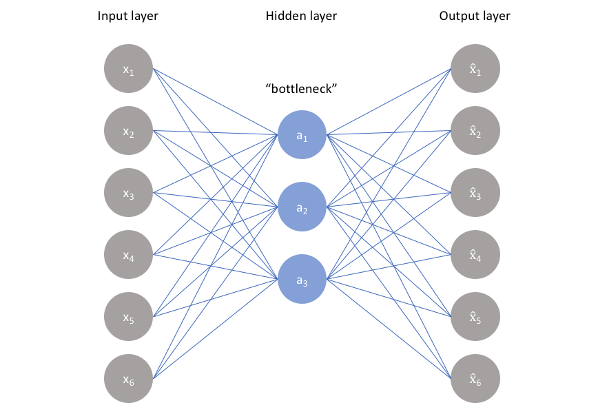
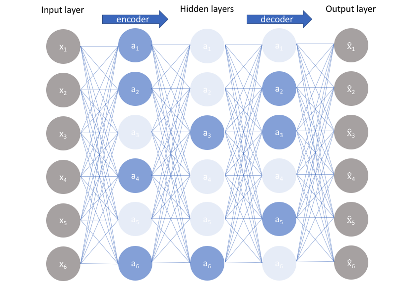
As visualized above, we can take an unlabeled dataset and frame it as a supervised learning problem tasked with outputting $\hat x$, a reconstruction of the original input $x$. This network can be trained by minimizing the reconstruction error, ${\cal L}\left( {x,\hat x} \right)$, which measures the differences between our original input and the consequent reconstruction. The bottleneck is a key attribute of our network design; without the presence of an information bottleneck, our network could easily learn to simply memorize the input values by passing these values along through the network (visualized below).
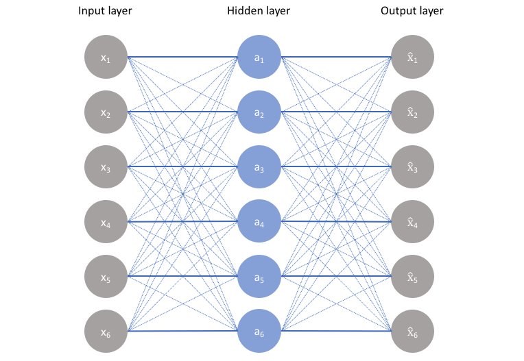
A bottleneck constrains the amount of information that can traverse the full network, forcing a learned compression of the input data.
Note: In fact, if we were to construct a linear network (ie. without the use of nonlinear activation functions at each layer) we would observe a similar dimensionality reduction as observed in PCA. See Geoffrey Hinton's discussion of this here.
The ideal autoencoder model balances the following:
- Sensitive to the inputs enough to accurately build a reconstruction.
- Insensitive enough to the inputs that the model doesn't simply memorize or overfit the training data.
This trade-off forces the model to maintain only the variations in the data required to reconstruct the input without holding on to redundancies within the input. For most cases, this involves constructing a loss function where one term encourages our model to be sensitive to the inputs (ie. reconstruction loss ${\cal L}\left( {x,\hat x} \right)$) and a second term discourages memorization/overfitting (ie. an added regularizer).
$$ {\cal L}\left( {x,\hat x} \right) + regularizer $$
We'll typically add a scaling parameter in front of the regularization term so that we can adjust the trade-off between the two objectives.
In this post, I'll discuss some of the standard autoencoder architectures for imposing these two constraints and tuning the trade-off; in a follow-up post I'll discuss variational autoencoders which builds on the concepts discussed here to provide a more powerful model.
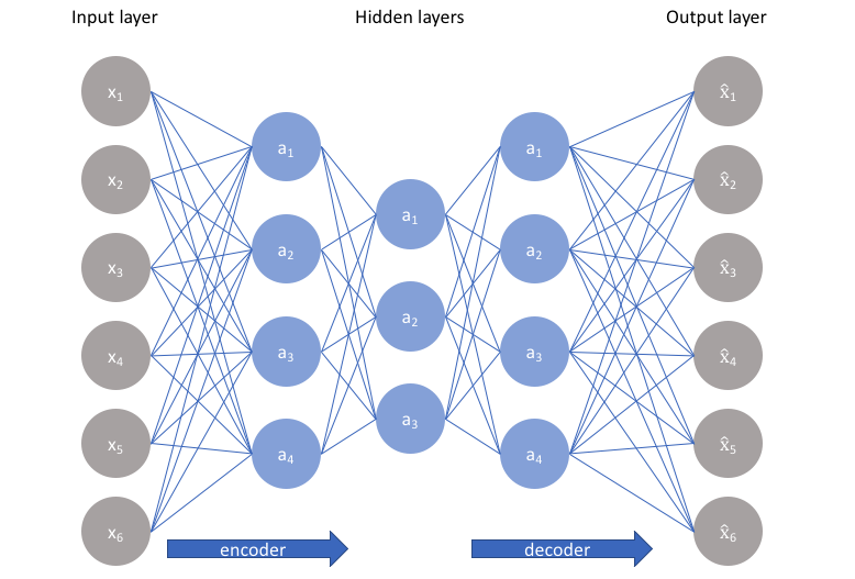
Undercomplete autoencoder
The simplest architecture for constructing an autoencoder is to constrain the number of nodes present in the hidden layer(s) of the network, limiting the amount of information that can flow through the network. By penalizing the network according to the reconstruction error, our model can learn the most important attributes of the input data and how to best reconstruct the original input from an "encoded" state. Ideally, this encoding will learn and describe latent attributes of the input data.
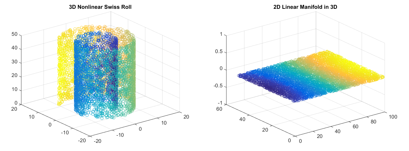
Because neural networks are capable of learning nonlinear relationships, this can be thought of as a more powerful (nonlinear) generalization of PCA. Whereas PCA attempts to discover a lower dimensional hyperplane which describes the original data, autoencoders are capable of learning nonlinear manifolds (a manifold is defined in simple terms as a continuous, non-intersecting surface). The difference between these two approaches is visualized below.
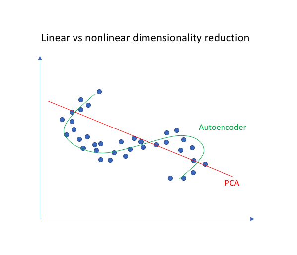
For higher dimensional data, autoencoders are capable of learning a complex representation of the data (manifold) which can be used to describe observations in a lower dimensionality and correspondingly decoded into the original input space.
An undercomplete autoencoder has no explicit regularization term - we simply train our model according to the reconstruction loss. Thus, our only way to ensure that the model isn't memorizing the input data is the ensure that we've sufficiently restricted the number of nodes in the hidden layer(s).
For deep autoencoders, we must also be aware of the capacity of our encoder and decoder models. Even if the "bottleneck layer" is only one hidden node, it's still possible for our model to memorize the training data provided that the encoder and decoder models have sufficient capability to learn some arbitrary function which can map the data to an index.
Given the fact that we'd like our model to discover latent attributes within our data, it's important to ensure that the autoencoder model is not simply learning an efficient way to memorize the training data. Similar to supervised learning problems, we can employ various forms of regularization to the network in order to encourage good generalization properties; these techniques are discussed below.
Sparse autoencoders
Sparse autoencoders offer us an alternative method for introducing an information bottleneck without requiring a reduction in the number of nodes at our hidden layers. Rather, we'll construct our loss function such that we penalize activations within a layer. For any given observation, we'll encourage our network to learn an encoding and decoding which only relies on activating a small number of neurons. It's worth noting that this is a different approach towards regularization, as we normally regularize the weights of a network, not the activations.
A generic sparse autoencoder is visualized below where the opacity of a node corresponds with the level of activation. It's important to note that the individual nodes of a trained model which activate are data-dependent, different inputs will result in activations of different nodes through the network.
One result of this fact is that we allow our network to sensitize individual hidden layer nodes toward specific attributes of the input data. Whereas an undercomplete autoencoder will use the entire network for every observation, a sparse autoencoder will be forced to selectively activate regions of the network depending on the input data. As a result, we've limited the network's capacity to memorize the input data without limiting the networks capability to extract features from the data. This allows us to consider the latent state representation and regularization of the network separately, such that we can choose a latent state representation (ie. encoding dimensionality) in accordance with what makes sense given the context of the data while imposing regularization by the sparsity constraint.
There are two main ways by which we can impose this sparsity constraint; both involve measuring the hidden layer activations for each training batch and adding some term to the loss function in order to penalize excessive activations. These terms are:
- L1 Regularization: We can add a term to our loss function that penalizes the absolute value of the vector of activations $a$ in layer $h$ for observation $i$, scaled by a tuning parameter $\lambda$.
$$ {\cal L}\left( {x,\hat x} \right) + \lambda \sum\limits_i {\left| {a_i^{\left( h \right)}} \right|} $$
- KL-Divergence: In essence, KL-divergence is a measure of the difference between two probability distributions. We can define a sparsity parameter $\rho$ which denotes the average activation of a neuron over a collection of samples. This expectation can be calculated as $ {{\hat \rho }_ j} = \frac{1}{m}\sum\limits_{i} {\left[ {a_i^{\left( h \right)}\left( x \right)} \right]} $ where the subscript $j$ denotes the specific neuron in layer $h$, summing the activations for $m$ training observations denoted individually as $x$. In essence, by constraining the average activation of a neuron over a collection of samples we're encouraging neurons to only fire for a subset of the observations. We can describe $\rho$ as a Bernoulli random variable distribution such that we can leverage the KL divergence (expanded below) to compare the ideal distribution $\rho$ to the observed distributions over all hidden layer nodes $\hat \rho$.
$$ {\cal L}\left( {x,\hat x} \right) + \sum\limits_{j} {KL\left( {\rho ||{{\hat \rho }_ j}} \right)} $$
Note: A Bernoulli distribution is "the probability distribution of a random variable which takes the value 1 with probability $p$ and the value 0 with probability $q=1-p$". This corresponds quite well with establishing the probability a neuron will fire.
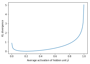
The KL divergence between two Bernoulli distributions can be written as $\sum\limits_{j = 1}^{{l^{\left( h \right)}}} {\rho \log \frac{\rho }{{{{\hat \rho }_ j}}}} + \left( {1 - \rho } \right)\log \frac{{1 - \rho }}{{1 - {{\hat \rho }_ j}}}$. This loss term is visualized below for an ideal distribution of $\rho = 0.2$, corresponding with the minimum (zero) penalty at this point.
Denoising autoencoders
So far I've discussed the concept of training a neural network where the input and outputs are identical and our model is tasked with reproducing the input as closely as possible while passing through some sort of information bottleneck. Recall that I mentioned we'd like our autoencoder to be sensitive enough to recreate the original observation but insensitive enough to the training data such that the model learns a generalizable encoding and decoding. Another approach towards developing a generalizable model is to slightly corrupt the input data but still maintain the uncorrupted data as our target output.
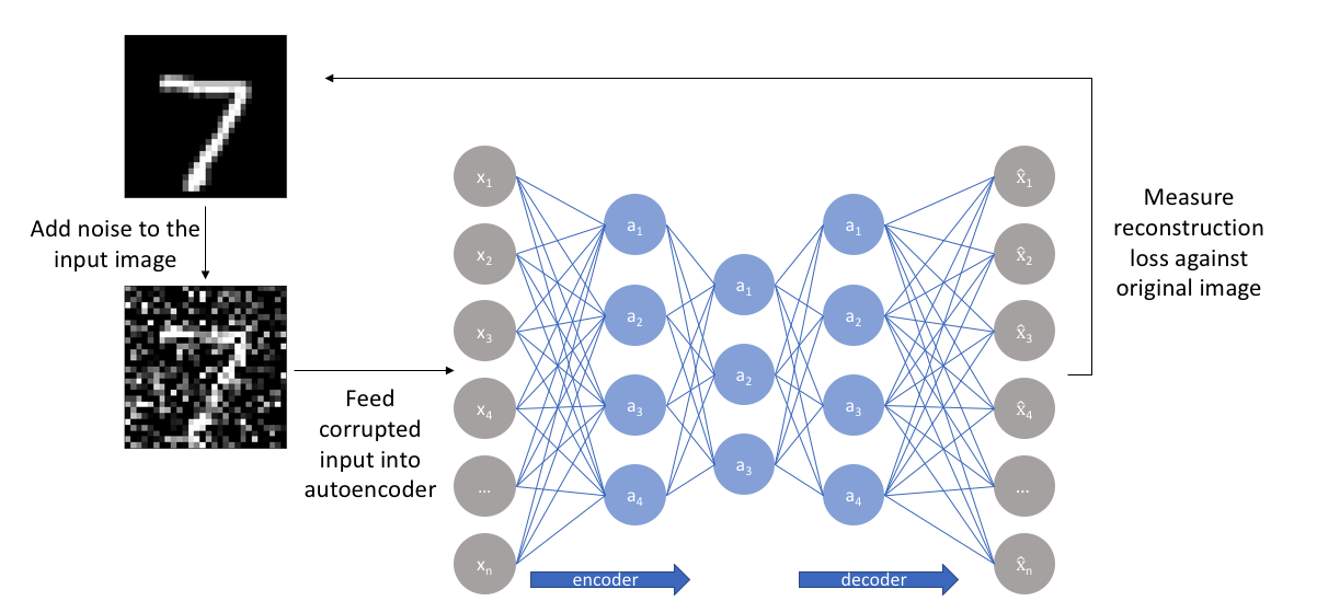
With this approach, our model isn't able to simply develop a mapping which memorizes the training data because our input and target output are no longer the same. Rather, the model learns a vector field for mapping the input data towards a lower-dimensional manifold (recall from my earlier graphic that a manifold describes the high density region where the input data concentrates); if this manifold accurately describes the natural data, we've effectively "canceled out" the added noise.
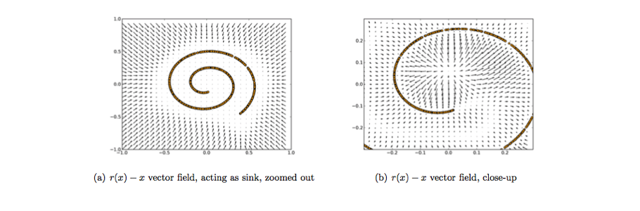
The above figure visualizes the vector field described by comparing the reconstruction of $x$ with the original value of $x$. The yellow points represent training examples prior to the addition of noise. As you can see, the model has learned to adjust the corrupted input towards the learned manifold.
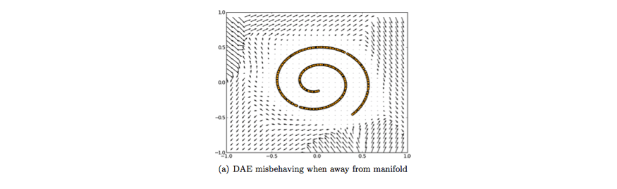
It's worth noting that this vector field is typically only well behaved in the regions where the model has observed during training. In areas far away from the natural data distribution, the reconstruction error is both large and does not always point in the direction of the true distribution.
Contractive autoencoders
One would expect that for very similar inputs, the learned encoding would also be very similar. We can explicitly train our model in order for this to be the case by requiring that the derivative of the hidden layer activations are small with respect to the input. In other words, for small changes to the input, we should still maintain a very similar encoded state. This is quite similar to a denoising autoencoder in the sense that these small perturbations to the input are essentially considered noise and that we would like our model to be robust against noise. Put in other words (emphasis mine), "denoising autoencoders make the reconstruction function (ie. decoder) resist small but finite-sized perturbations of the input, while contractive autoencoders make the feature extraction function (ie. encoder) resist infinitesimal perturbations of the input."
Because we're explicitly encouraging our model to learn an encoding in which similar inputs have similar encodings, we're essentially forcing the model to learn how to contract a neighborhood of inputs into a smaller neighborhood of outputs. Notice how the slope (ie. derivative) of the reconstructed data is essentially zero for local neighborhoods of input data.
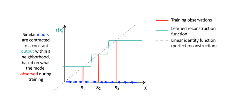
Image credit (modified)
We can accomplish this by constructing a loss term which penalizes large derivatives of our hidden layer activations with respect to the input training examples, essentially penalizing instances where a small change in the input leads to a large change in the encoding space.
In fancier mathematical terms, we can craft our regularization loss term as the squared Frobenius norm ${\left\lVert A \right\rVert_F}$ of the Jacobian matrix ${\bf{J}}$ for the hidden layer activations with respect to the input observations. A Frobenius norm is essentially an L2 norm for a matrix and the Jacobian matrix simply represents all first-order partial derivatives of a vector-valued function (in this case, we have a vector of training examples).
For $m$ observations and $n$ hidden layer nodes, we can calculate these values as follows.
$${\left\lVert A \right\rVert_F}= \sqrt {\sum\limits_{i = 1}^m {\sum\limits_{j = 1}^n {{{\left| {{a_{ij}}} \right|}^2}} } } $$
Written more succinctly, we can define our complete loss function as
$$ {\cal L}\left( {x,\hat x} \right) + \lambda {\sum\limits_i {\left\lVert {{\nabla _ x}a_i^{\left( h \right)}\left( x \right)} \right\rVert} ^2} $$
where ${{\nabla_x}a_i^{\left( h \right)}\left( x \right)}$ defines the gradient field of our hidden layer activations with respect to the input $x$, summed over all $i$ training examples.
Summary
An autoencoder is a neural network architecture capable of discovering structure within data in order to develop a compressed representation of the input. Many different variants of the general autoencoder architecture exist with the goal of ensuring that the compressed representation represents meaningful attributes of the original data input; typically the biggest challenge when working with autoencoders is getting your model to actually learn a meaningful and generalizable latent space representation.
Because autoencoders learn how to compress the data based on attributes (ie. correlations between the input feature vector) discovered from data during training, these models are typically only capable of reconstructing data similar to the class of observations of which the model observed during training.
Applications of autoencoders include:
- Anomaly detection
- Data denoising (ex. images, audio)
- Image inpainting
- Information retrieval
Further reading
Lectures/notes
- Unsupervised feature learning - Stanford
- Sparse autoencoder - Andrew Ng CS294A Lecture notes
- UC Berkley Deep Learning Decall Fall 2017 Day 6: Autoencoders and Representation Learning
Blogs/videos
Papers/books