Normalizing your data (specifically, input and batch normalization).
In this post, I'll discuss considerations for normalizing your data - with a specific focus on neural networks. In order to understand the concepts discussed, it's important to have an understanding of gradient descent.

In this post, I'll discuss considerations for normalizing your data - with a specific focus on neural networks. In order to understand the concepts discussed, it's important to have an understanding of gradient descent.
As a quick refresher, when training neural networks we'll feed in observations and compare the expected output to the true output of the network. We'll then use gradient descent to update the parameters of the model in the direction which will minimize the difference between our expected (or ideal) outcome and the true outcome. In other words, we're attempting to minimize the error we observe in our model's predictions.
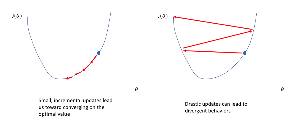
The exact manner by which we update our model parameters will depend on the variant of gradient descent optimization techniques we select (stochastic gradient descent, RMSProp, Adam, etc.) but all of these update techniques will scale the magnitude of our parameter update by a learning rate. This rate ensures that we aren't changing the parameter too drastically such that we overshoot our update and fail to find the optimal value.
Ultimately, gradient descent is a search among a loss function surface in an attempt to find the values for each parameter such that the loss function is minimized. In other words, we're looking for the lowest value on the loss function surface. In my post on gradient descent, I discussed a few advanced techniques for efficiently updating our parameter values such that we can avoid getting stuck at saddle points. However, we can also improve the actual topology of our loss function by ensuring all of the parameters exist on the same scale.
Note: Understanding the topology of loss functions, and how network design affects this topology, is a current area of research in the field.
The important thing to remember throughout this discussion is that our loss function surface is characterized by the parameter values in the network. When visualizing this topology, each parameter will represent a dimension of which a range of values will have a resulting affect on the value of our loss function. Unfortunately, this becomes rather tricky to visualize once you extend beyond two parameters (a dimension characterized by each parameter, and the third dimension representing the value of the loss function).
In the above image, we're visualizing the loss function of a model parameterized by two weights (the x and y dimensions) with the z dimension representing the corresponding "error" (loss) of the network.
This 3D visualization is often also represented by a 2D contour plot.
What's the problem with unnormalized data?
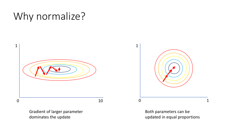
Let's take a second to imagine a scenario in which you have a very simple neural network with two inputs. The first input value, $x_1$, varies from 0 to 1 while the second input value, $x_2$, varies from 0 to 0.01. Since your network is tasked with learning how to combine these inputs through a series of linear combinations and nonlinear activations, the parameters associated with each input will also exist on different scales.
Unfortunately, this can lead toward an awkward loss function topology which places more emphasis on certain parameter gradients.
More discussion on this subject found here.
By normalizing all of our inputs to a standard scale, we're allowing the network to more quickly learn the optimal parameters for each input node.
Additionally, it's useful to ensure that our inputs are roughly in the range of -1 to 1 to avoid weird mathematical artifacts associated with floating point number precision. In short, computers lose accuracy when performing math operations on really large or really small numbers. Moreover, if your inputs and target outputs are on a completely different scale than the typical -1 to 1 range, the default parameters for your neural network (ie. learning rates) will likely be ill-suited for your data.
Implementation
It's a common practice to scale your data inputs to have zero mean and unit variance. This is known as the standard scaler approach.
However, you may opt for a different normalization strategy. For example, it's common for image data to simply be scaled by 1/255 so that the pixel intensity range is bound by 0 and 1.
Batch normalization
Normalizing the input of your network is a well-established technique for improving the convergence properties of a network. A few years ago, a technique known as batch normalization was proposed to extend this improved loss function topology to more of the parameters of the network.
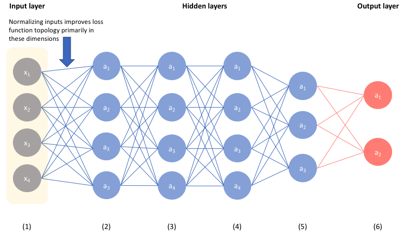
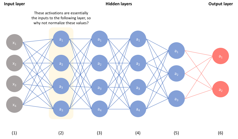
If we were to consider the above network as an example, normalizing our inputs will help ensure that our network can effectively learn the parameters in the first layer.
However, consider the fact that the second layer of our network accepts the activations from our first layer as input. Thus, by extending the intuition established in the previous section, one could posit that normalizing these values will help the network more effectively learn the parameters in the second layer.
By ensuring the activations of each layer are normalized, we can simplify the overall loss function topology. This is especially helpful for the hidden layers of our network, since the distribution of unnormalized activations from previous layers will change as the network evolves and learns more optimal parameters. Thus, by normalizing each layer, we're introducing a level of orthogonality between layers - which generally makes for an easier learning process.
Implementation
To summarize, we'd like to normalize the activations of a given layer such that we improve learning of the weights which connect the next layer. In practice, people will typically normalize the value of ${z^{\left[ l \right]}}$ rather than ${a^{\left[ l \right]}}$ - although sometimes debated whether we should normalize before or after activation.
Given a vector of linear combinations from the previous layer ${z^{\left[ l \right]}}$ for each observation $i$ in a dataset, we can calculate the mean and variance as:
$$ \mu = \frac{1}{m}\sum\limits_i {z_i^{\left[ l \right]}} $$
$$ {\sigma ^2} = \frac{1}{m}{\sum\limits_i {\left( {z_i^{\left[ l \right]} - \mu } \right)} ^2} $$
Using these values, we can normalize the vectors ${z^{\left[ l \right]}}$ as follows.
$$z_{norm}^{\left( i \right)} = \frac{{{z^{\left( i \right)}} - \mu }}{{\sqrt {{\sigma ^2} + \varepsilon } }}$$
We add a very small number $\epsilon$ to prevent the chance of a divide by zero error.
However, it may not be the case that we always want to normalize $z$ to have zero mean and unit variance. In fact, this would perform poorly for some activation functions such as the sigmoid function. Thus, we'll allow our normalization scheme to learn the optimal distribution by scaling our normalized values by $\gamma$ and shifting by $\beta$.
$${{\tilde z}^{\left( i \right)}} = \gamma z_{norm}^{\left( i \right)} + \beta $$
In other words, we've now allowed the network to normalize a layer into whichever distribution is most optimal for learning.
One result of batch normalization is that we no longer need a bias vector for a batch normalized layer given that we are already shifting the normalized $z$ values with the $\beta$ parameter.
Note: $\mu$ and ${\sigma ^2}$ are calculated on a per-batch basis while $\gamma$ and $\beta$ are learned parameters used across all batches.
Summary
Ultimately, batch normalization allows us to build deeper networks without the need for exponentially longer training times. This is a result of introducing orthogonality between layers such that we avoid shifting distributions in activations as the parameters in earlier layers are updated.
Further reading
- Batch Normalization: Accelerating Deep Network Training by Reducing Internal Covariate Shift
- How Does Batch Normalization Help Optimization? (No, It Is Not About Internal Covariate Shift)
- CS231n Winter 2016: Lecture 5: Neural Networks Part 2
- Understanding the backward pass through Batch Normalization Layer
- Layer Normalization
The paper that introduced Batch Norm https://t.co/vkT0LioKHc combines clear intuition with compelling experiments (14x speedup on ImageNet!!)
— David Page (@dcpage3) September 11, 2019
So why has 'internal covariate shift' remained controversial to this day?
Thread 👇 pic.twitter.com/L0BBmo0q4t