Decision trees.

Decision trees are one of the oldest and most widely-used machine learning models, due to the fact that they work well with noisy or missing data, can easily be ensembled to form more robust predictors, and are incredibly fast at runtime. Moreover, you can directly visual your model's learned logic, which means that it's an incredibly popular model for domains where model interpretability is important.
Decision trees are pretty easy to grasp intuitively, let's look at an example.
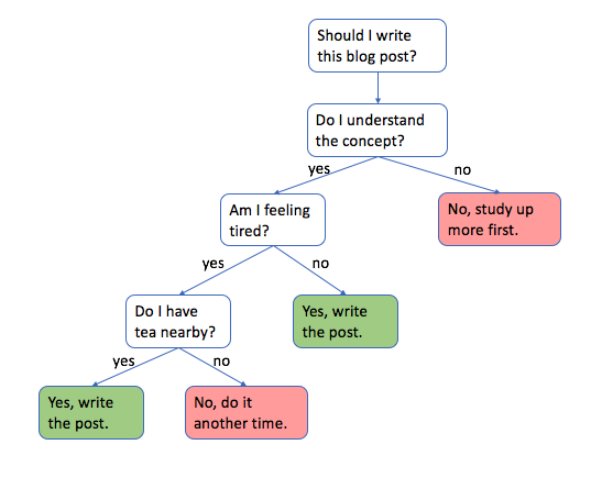
Note: decision trees are used by starting at the top and going down, level by level, according to the defined logic. This is known as recursive binary splitting.
For those wondering – yes, I'm sipping tea as I write this post late in the evening. Now let's dive in!
Classification
Let's look at a two-dimensional feature set and see how to construct a decision tree from data. The goal is to construct a decision boundary such that we can distinguish from the individual classes present.
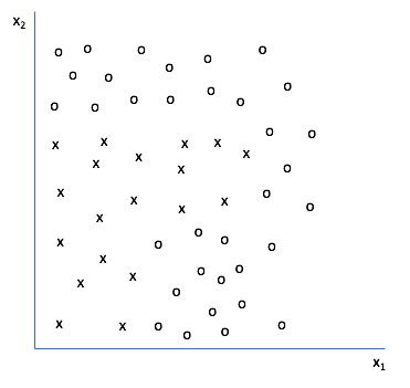
Any ideas on how we could make a decision tree to classify a new data point as "x" or "o"? Here's what I did.
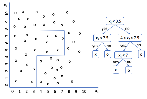
Run through a few scenarios and see if you agree. Look good? Cool. So now we have a decision tree for this data set; the only problem is that I created the splitting logic. It'd be much better if we could get a machine to do this for us. But how?
If you analyze what we're doing from an abstract perspective, we're taking a subset of the data, and deciding the best manner to split the subset further. Our initial subset was the entire data set, and we split it according to the rule $x_1 < 3.5$. Then, for each subset, we performed additional splitting until we were able to correctly classify every data point.
Information gain and entropy
How do we judge the best manner to split the data? Simply, we want to split the data in a manner which provides us the most amount of information - in other words, maximizing information gain. Going back to the previous example, we could have performed our first split at $x_1 < 10$. However, this would essentially be a useless split and provide zero information gain. In order to mathematically quantify information gain, we introduce the concept of entropy.
[\mathop - \sum \limits _i^{} {p _i}{\log _2}\left( {{p _i}} \right)]
Entropy may be calculated as a summation over all classes where $p_i$ is the fraction of data points within class $i$. This essentially represents the impurity, or noisiness, of a given subset of data. A homogenous dataset will have zero entropy, while a perfectly random dataset will yield a maximum entropy of 1. With this knowledge, we may simply equate the information gain as a reduction in noise.
Here, we're comparing the noisiness of the data before splitting the data (parent) and after the split (children). If the entropy decreases due to a split in the dataset, it will yield an information gain. A decision tree classifier will make a split according to the feature which yields the highest information gain. This is a recursive process; stopping criterion for this process include continuing to split the data until (1) the tree is capable of correctly classifying every data point, (2) the information gain from further splitting drops below a given threshold, (3) a node has fewer samples than some specified threshold, (4) the tree has reached a maximum depth, or (5) another parameter similarly calls for the end of splitting. To learn more about this process, read about the ID3 algorithm.
Techniques to avoid overfitting
Often you may find that you've overfitted your model to the data, which is often detrimental to the model's performance when you introduce new data. To prevent this overfitting, one thing you could do is define some parameter which ends the recursive splitting process. As I mentioned earlier, this may be a parameter such as maximum tree depth or minimum number of samples required in a split. Controlling these model hyperparameters is the easiest way to counteract overfitting.
You could also simply perform a significance test when considering a new split in the data, and if the split does not supply statistically significant information (obtained via a significance test), then you will not perform any further splits on a given node.
Another technique is known as pruning. Here, we grow a decision tree fully on your training dataset and then go back and evaluate its performance on a new validation dataset. For each node, we evaluate whether or not it's split was useful or detrimental to the performance on the validation dataset. We then remove those nodes which caused the greatest detriment to the decision tree performance.
Degenerate splits
Evaluating a split using information gain can pose a problem at times; specifically, it has a tendency to favor features which have a high number of possible values. Say I have a data set that determines whether or not I choose to go sailing for the month of June based on features such as temperature, wind speed, cloudiness, and day of the month. If I made a decision tree with 30 child nodes (Day 1, Day 2, ..., Day 30) I could easily build a tree which accurately partitions my data. However, this is a useless feature to split based on because the second I enter the month of July (outside of my training data set), my decision tree has no idea whether or not I'm likely to go sailing. One way to circumvent this is to assign a cost function (in this case, the gain ratio) to prevent our algorithm from choosing attributes which provide a large number of subsets.
Example code
Here's an example implementation of a Decision Tree Classifier for classifying the flower species dataset we've studied previously.
import pandas as pd
from sklearn import datasets
from sklearn.tree import DecisionTreeClassifier
from sklearn.model_selection import train_test_split

iris = datasets.load_iris()      # ['target_names', 'data', 'target', 'DESCR', 'feature_names']
features = pd.DataFrame(iris.data)
labels = pd.DataFrame(iris.target)

### create classifier
clf = DecisionTreeClassifier(criterion='entropy')

### split data into training and testing datasets
features_train, features_test, labels_train, labels_test = train_test_split(features, labels, test_size=0.4, random_state=0)

### fit the classifier on the training features and labels
clf.fit(features_train, labels_train)

### use the trained classifier to predict labels for the test features
pred = clf.predict(features_test)

### calculate and return the accuracy on the test data
from sklearn.metrics import accuracy_score
accuracy = accuracy_score(labels_test, pred)

### visualize the decision tree
### you'll need to have graphviz and pydot installed on your computer
from IPython.display import Image
from sklearn.externals.six import StringIO
import pydot
from sklearn import tree

dot_data = StringIO()
tree.export_graphviz(clf, out_file=dot_data)
graph = pydot.graph_from_dot_data(dot_data.getvalue())
Image(graph[0].create_png())
Without any parameter tuning we see an accuracy of 94.9%, not too bad! The decision tree classifier in sklearn has an exhaustive set of parameters which allow for maximum control over your classifier. These parameters include: criterion for evaluating a split (this blog post talked about using entropy to calculate information gain, however, you can also use something known as Gini impurity), maximum tree depth, minimum number of samples required at a leaf node, and many more.
Regression
Regression models, in the general sense, are able to take variable inputs and predict an output from a continuous range. However, decision tree regressions are not capable of producing continuous output. Rather, these models are trained on a set of examples with outputs that lie in a continuous range. These training examples are partitioned in the decision tree and new examples that end in a given node will take on the mean of the training example values that reside in the same node.
It looks something like this.
Alright, but how do we get there? As I mentioned before, the general process is very similar to a decision tree classifier with a few small changes.
Determining the optimal split
We'll still build our tree recursively, making splits on the data as we go, but we need a new method for determining the optimal split. For classification, we used information entropy (you can also use the Gini index or Chi-square method) to figure out which split provided the biggest gain in information about the new example's class. For regression, we're not trying to predict a class, but rather we're expected the generate an output given the input criterion. Thus, we'll need a new method for determining optimal fit.
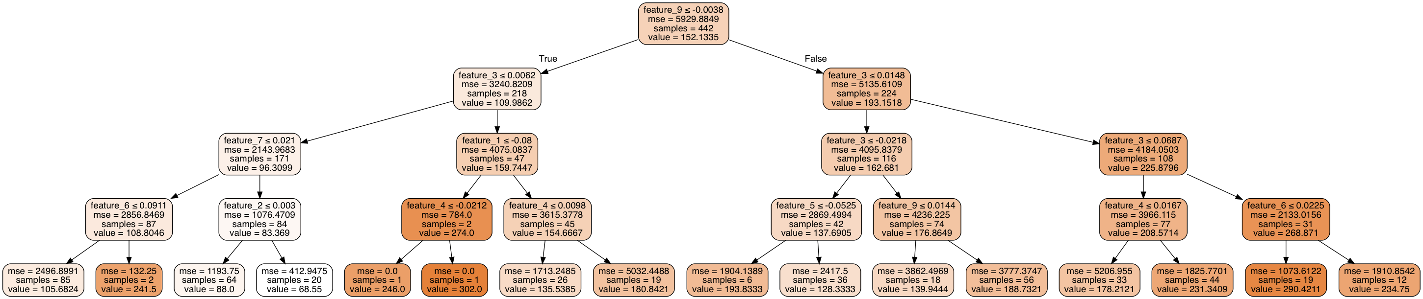
One way to do this is to measure whether or not a split will result in a reduction of variance within the data. If a split is useful, its combined weighted variance of the child nodes will be less than the original variance of the parent node. We can continue to make recursive splits on our dataset until we've effectively reduced the overall variance below a certain threshold, or upon reaching another stopping parameter (such as reaching a defined maximum depth). Notice how the mean squared error decreases as you step through the decision tree.
Avoiding overfitting
The techniques for preventing overfitting remain largely the same as for decision tree classifiers. However, it seems that not many people actually take the time to prune a decision tree for regression, but rather they elect to use a random forest regressor (a collection of decision trees) which are less prone to overfitting and perform better than a single optimized tree. The common argument for using a decision tree over a random forest is that decision trees are easier to interpret, you simply look at the decision tree logic. However, in a random forest, you're not going to want to study the decision tree logic of 500 different trees. Luckily for us, there are still ways to maintain interpretability within a random forest without studying each tree manually.
Implementation
Here's the code I used to generate the graphic above.
from sklearn import datasets
# Load the diabetes dataset
diabetes = datasets.load_diabetes()

import pandas as pd

features = pd.DataFrame(diabetes.data, columns = ["feature_1", "feature_2", "feature_3", "feature_4", "feature_5", "feature_6", "feature_7", "feature_8", "feature_9", "feature_10"])
target = pd.DataFrame(diabetes.target)

from sklearn.tree import DecisionTreeRegressor
regressor = DecisionTreeRegressor(max_depth = 4)
regressor.fit(features, target)

from IPython.display import Image
from sklearn.externals.six import StringIO
import pydot
from sklearn import tree

dot_data = StringIO()
tree.export_graphviz(regressor, out_file=dot_data,
    feature_names=features.columns,
    class_names=target.columns,
    filled=True, rounded=True,
    special_characters=True)
graph = pydot.graph_from_dot_data(dot_data.getvalue())
Image(graph[0].create_png())
Further reading
Brandon Rohrer: How decision trees work
An incredible interactive visualization of decision trees