Identifying related bodies of text using TF-IDF vectorization.

Term frequency-inverse document frequency (TF-IDF) vectorization is a mouthful to say, but it's also a simple and convenient way to characterize bodies of text. Due to its simplicity, this method scales better than some other topic modeling techniques (latent dirichlet allocation, probabilistic latent semantic indexing) when dealing with large datasets.
TF-IDF Vectorization
Let's say we have a collection of documents:
- Document 1: "TF-IDF vectorization is a useful tool for text analytics. It allows you to quantify the similarity of different documents."
- Document 2: "You can use cosine similarity to analyze TF-IDF vectors and cluster text documents based on their content."
- Document 3: "The weather today is looking quite bleak. It's a great day to write a blog post!"
It's clear to us that Document 1 and 2 are related, but how can we train an algorithm to identify this? First, let's split up the documents into a collection of words. This is known as tokenization - we'll split up the sentences into a list of words, removing capitalization (so "You" and "you" are treated as the same thing) and ignoring punctuation. See the pseudo-code example below.
>> tokenize("TF-IDF vectorization is a useful tool for text analytics. It allows you to quantify the similarity of different documents.")

"TFIDF", "vectorization", "is", "a", "useful", "tool", "for", "text", "analytics", "it", "allows", "you", "to", "quantify", "the", "similarity", "of", "different", "documents"
Term Frequency
Term frequency refers to how often a term (or token) occurs within a given document. Since my example documents are quite small, we don't observe a term that appears more than once. But if I treated an entire blog post (say, the one you're currently reading) as a document, you could see how terms such as "TFIDF" and "similarity" would appear more often than terms such as "blog." In short, term frequency describes how popular a term is within a single document.
Inverse Document Frequency
Document frequency counts the number of occurrences for each term across all documents. However, if a term is popular across all documents, it doesn't provide much information relative to a single document. The token "you" might appear often and have a high term frequency for a given document, but it likely appears often across all documents so it does little to provide any information. An extreme case of this are stopwords, which are terms such as "a", "the", "you", and "like" which usually provide so little information they are discarded upon tokenization. Thus, we calculate the inverse document frequency so that the terms that appear most often are weighted down. Another way of thinking about the IDF is that it establishes a scoring mechanism for the usefulness of a given term - higher scores mean more information is present. In short, inverse document frequency describes how unique a term is across the collection of documents.
Let's imagine that my document examples were each a paragraph long and the following table represents how often a few terms occur in each document.
Term Counts
The rows in these tables can be represented as N-dimensional term frequency vectors where the last row represents the document frequency. To find the TF-IDF vector for each document, we simply normalize the term frequency and inverse document frequency vectors and multiply them together.
Notes: Although this example uses linear frequency to help visualize how the pieces fit together, in practice you should use the log-frequency. Log-frequency lessens the difference between large term counts (ie. 1 vs 20 is treated as a larger difference than 100 vs 150). Also, this is element-wise multiplication. The TF score for "similarity" is multiplied by the IDF score for "similarity."
Cosine Similarity
Now that we have a TF-IDF vector for each document, we can quantify the similarity between two vectors using cosine similarity. The image below is quite instructive for providing the motivation behind this technique.
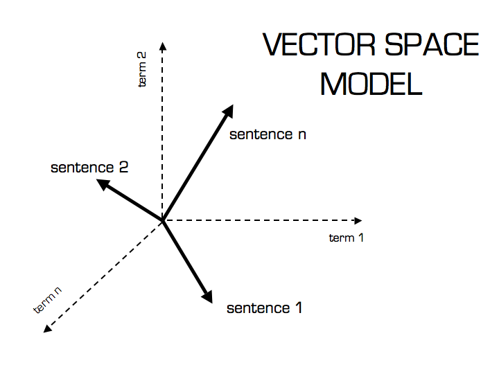
Thus, if two documents contain similar language (tokens) they will be closer together in the visualized N-dimensional vector space. We can calculate the cosine of the two vectors to determine how close the vectors are with respect to their orientation. The reason we take the cosine of the angle between two vectors rather than just measuring the distance between vectors is illustrated below.
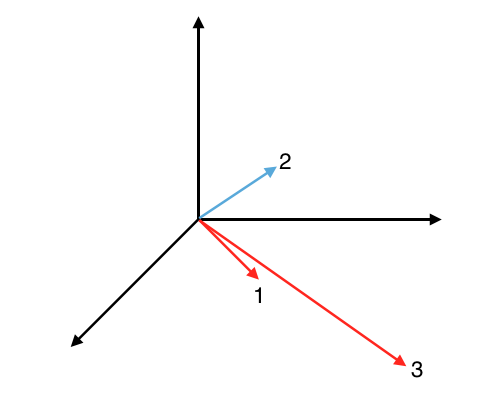
Although the two red vectors are very different in magnitude, they appear much more similar than vectors 1 and 2 (which are closer in distance.) To account for varying lengths in documents, we also normalize each TF-IDF vector with respect to its length. After length-normalizing the two TF-IDF vectors you wish to compare, you can simply take the dot product to find the cosine similarity
where q and d are the two documents and n represents the total number of terms in the global documents vocabulary.
Note: these TF-IDF vectors are generally very sparse, as an individual document will only contain a small subset of the vocabulary found across the collection of documents. If you don't know how to optimize operations dealing with sparse vectors, I'd recommend using SKLearn's TF-IDF vectorizer. In fact, I'd recommend that module regardless because it works really well and has a number of features, such as tokenization, n-grams (which creates tokens for collections of words in addition to individual words), and stopword removal.
Example Code
Here's a quick example using SKLearn's TF-IDF vectorizer module.
from sklearn.feature_extraction.text import TfidfVectorizer
from sklearn.metrics.pairwise import cosine_similarity

tfidf_vectorizer = TfidfVectorizer()
print "Fitting TF-IDF matrix..."
tfidf_matrix = tfidf_vectorizer.fit_transform(documents)
print "Calculating cosine similarity..."
dist = 1 - cosine_similarity(tfidf_matrix)