Boosted trees.

Boosting is an iterative ensembling process where models are trained in a sequential order. These models are known as "weak learners" as they are simple prediction rules which only perform slightly better than a random guess (ie. slightly better than 50% accuracy). The general concept behind boosting is to focus on the "hard" examples, or the examples that the model fails to predict correctly with confidence. These examples are given more emphasis by skewing the distribution of observations so that these examples are more likely to appear in a sample. As such, the next weak learner will focus more on getting these hard examples correct. Because your learner is always doing better than random, you'll always get some degree of information from each sequential training round. When all of the simple prediction rules are combined into one overarching model, a powerful predictor emerges.
One useful characteristic of boosted ensemble learners is that, provided you use simple learners, the ensemble model is very robust against overfitting. Typically, when training a model you run the danger of overfitting if you continue optimizing for total accuracy of the training data; this is why cross validation is important as it ensures that we'll still have a model that performs well when we feed it new data. A typical validation curve (plot of training score and cross-validation score as a function of iterative trainings) will diverge at some point when you've begun to overfit your data.
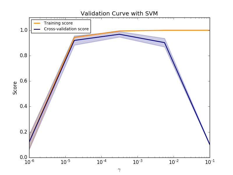
However, this divergence doesn't occur in boosting models, which is quite convenient. The reason is that boosting focuses its efforts on performing well for "hard" examples. For instance, think of the case for classification; "hard" examples are those which are close to the decision boundary, so the boosting algorithm will focus its efforts on doing a better job at separating these data points. What results is an increased margin between the observations on each side of the decision boundary. As we learned with support vector machines, large margin separators tend to generalize well and are not prone to overfitting.
AdaBoost
AdaBoost (adaptive boosting) is the most popular boosting technique, developed for classification (and later extended to regression). The general steps are as follows:
- Attach weights to each sample, initially achieving a uniform distribution. Given $m$ observations, we'll start off treating all of our data as equal. These weights are what we'll update in order to give more emphasis on the observations which perform poorly in our model.
[{w _1}\left( i \right) = \frac{1}{m}] - Train a weak learner, ${{h _t}\left( x \right)}$, on a random sample weighted by an initially uniform distribution, ${w _1}\left( i \right)$.
- Calculate the error associated with the learner, ${{h _t}\left( x \right)}$. We'll calculate error as the probability that the model misclassifies a data point; this will implicitly take into account the weighted distribution of observations.
[{\varepsilon _t} = P\left( {{h _t}\left( {{x _i}} \right) \ne {y _i}} \right)] - Score the model as a function of it's error. This equation is not a niave assertion, but derived from calculus in an attempt to figure a method which minimizes total error.
[{\alpha _t} = {\raise0.5ex\hbox{$\scriptstyle 1$}
\kern-0.1em/\kern-0.15em
\lower0.25ex\hbox{$\scriptstyle 2$}}\ln \frac{{1 - {\varepsilon _t}}}{{{\varepsilon _t}}}] - Recalculate the weights for each observation to form a new distribution. More emphasis will be placed on observations which are misclassified. $z _t$ serves as a normalization factor to ensure the weights add up to one (thus forming a distribution).
[{w _{t + 1}}\left( i \right) = {w _t}\left( i \right)\frac{{{e^{ - {\alpha _t}{y _i}{h _t}\left( {{x _i}} \right)}}}}{{{z _t}}}]
[{z _t} = 2\sqrt {{\varepsilon _t}\left( {1 - {\varepsilon _t}} \right)}] - Iteratively train models and recalculate distributions in an effort to place more emphasis on the observations which are not being modeled accurately.
In a sense, each sequential hypothesis will output a prediction for the class of $x _i$, either $-1$ or $1$. Our final model will combine these predictions, weighted according to how well the individual model performs (according to ${\alpha _t}$).
[{H _{final}} = {\mathop{\rm sgn}} \left( {\sum\limits _t {{\alpha _t}{h _t}\left( x \right)} } \right)]
Gradient Boosting (XGBoost)
Gradient boosting is a generalized approach of boosting which allows for the optimization of an arbitrarily-defined loss function. I'll be revisiting this blog post in the near future to provide a more detailed description of this technique.
Further reading
The Boosting Approach to Machine Learning:
An Overview
A Kaggle Master Explains Gradient Boosting