Support vector machines.

Today we'll be talking about support vector machines (SVM); this classifier works well in complicated feature domains, albeit requiring clear separation between classes. SVMs don't work well with noisy data, and the algorithm scales roughly cubic $O(n^3)$ to input depending on your implementation (sklearn's SVM fit time complexity is more than quadratic, so it won't be able to train quickly on large datasets (>10,000 examples).
Intuition
Before we get into any more details, I'd like to introduce a description of SVMs I saw on Reddit in an attempt to explain what it is to a 5-year-old.
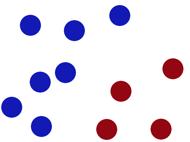
We have 2 colors of balls on the table that we want to separate.
http://i.imgur.com/zDBbD.png
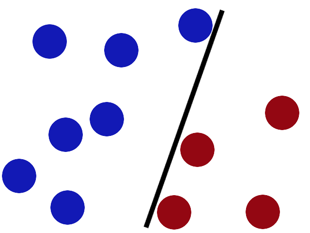
We get a stick and put it on the table, this works pretty well right?
http://i.imgur.com/aLZlG.png
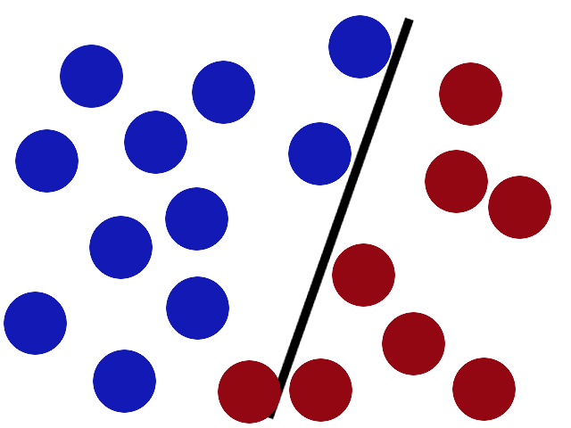
Some villain comes and places more balls on the table, it kind of works but one of the balls is on the wrong side and there is probably a better place to put the stick now.
http://i.imgur.com/kxWgh.png
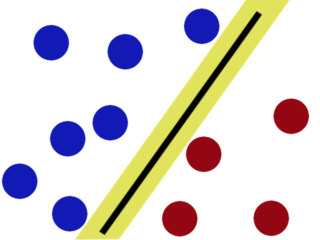
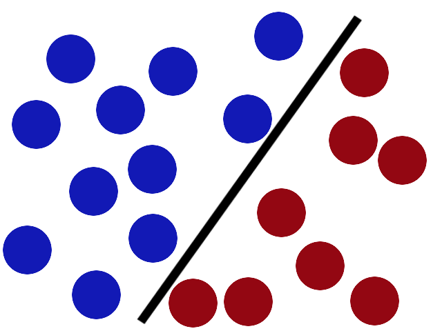
SVMs try to put the stick in the best possible place by having as big a gap on either side of the stick as possible.
http://i.imgur.com/ePy4V.png
Now when the villain returns the stick is still in a pretty good spot.
http://i.imgur.com/BWYYZ.png
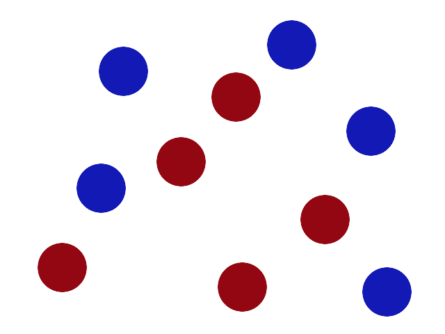
There is another trick in the SVM toolbox that is even more important. Say the villain has seen how good you are with a stick so he gives you a new challenge.
http://i.imgur.com/R9967.png
There’s no stick in the world that will let you split those balls well, so what do you do? You flip the table of course! Throwing the balls into the air. Then, with your pro ninja skills, you grab a sheet of paper and slip it between the balls.
http://i.imgur.com/WuxyO.png
Now, looking at the balls from where the villain is standing, they balls will look split by some curvy line.
http://i.imgur.com/gWdPX.png
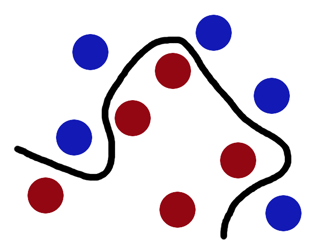
Boring adults call the balls data, the stick is a classifier, the biggest gap trick is called optimization, flipping the table is called kernelling and the piece of paper a hyperplane.
Sometimes it's best to keep things simple.
The model
As with logistic regression, and model-based classification in general, our goal is to determine some establishing decision boundary which is capable of separating the data into homogenous groups (ie. every example on the same of a decision boundary has the same label) using the features provided.
In my post on logistic regression, we established that it is possible to draw a line, $z\left( x \right)$, so that points on one side take on positive values and points on the opposite side take on negative values.
For example, in the following graph, $z = 6 - {x _1}$ represents a decision boundary for which any values of ${x _1} > 6$ will return a negative value for $z$ and any values of ${x _1} < 6$ will return a positive value for $z$. For the case where we have two features, our decision boundary happens to be a line. More generally, we'll refer to this boundary as a hyperplane- a subspace which consists of one less dimension than your feature space. Thus, if we were to draw a decision boundary for a dataset with three features, our boundary would be a plane.
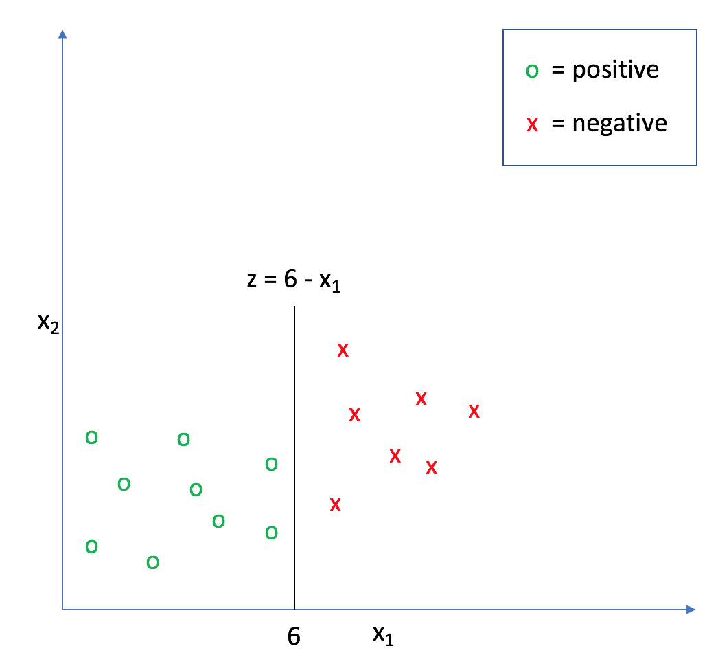
We further established that you can think of $z\left( x \right)$ as a measure of how far a certain data point exists from the decision boundary.
With logistic regression, we used the notation
[z(x) = {\theta ^T}x = {\theta _0}{x _0} + {\theta _1}{x _1} + {\theta _2}{x _2} + ... + {\theta _n}{x _n}]
where $x _0 = 1$ by convention to represent our linear model. For support vector machines, it is more convenient to separate the intercept term, $\theta _0$, from the rest of the parameters ${\theta _{1,2,...,n}}$ due to the calculations we'll do. The standard way of writing our model for a support vector machine is
[z(x) = {w^T}x + b ]
which expands to be
[z(x) = b + {w _1}{x _1} + {w _2}{x _2} + ... + {w _n}{x _n}]
where ${w^T}$ is equivalent to ${\theta _{1,2,...,n}^T}$ and $b$ is equivalent to $\theta _0$. This way, $x _0$ is implicitly defined to be equal to one.
More completely, we'll define our classification function, $g\left( z \right)$, as
which, combined with $z\left( x \right)$, yields our complete model for SVMs.
[{h_{w,b}}\left( x \right) = g\left( {z(x)} \right) = g\left( {{w^T}x + b} \right)]
Note: for SVMs we use class labels {-1, 1} instead of {0, 1} as we did in logistic regression.
Defining a margin
Remember, this decision boundary is established based on what our model can learn from the training dataset. However, we'd ultimately like for the model to perform well for new data, or at the very least the data in our testing dataset.
It makes somewhat intuitive sense that we can predict examples that lie far away from the decision boundary more confidently than those which lie close.
For example, given two new observations, $A$ and $B$, which example would you be more confident in classifying?
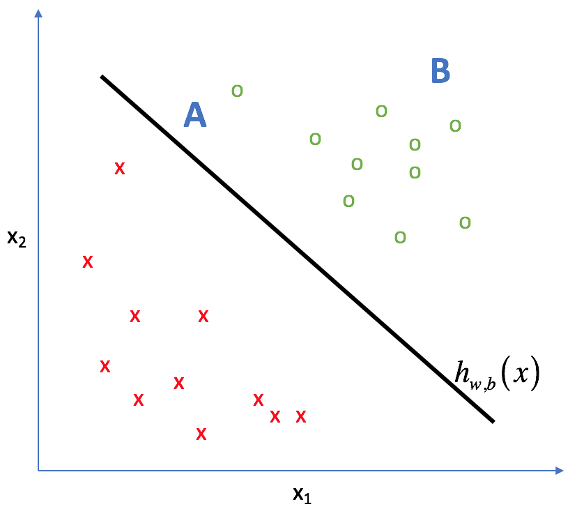
They're technically the same class, but I'd be much more comfortable predicting the class of $B$. The optimized hyperplane will change slightly when trained on different subsets of your data, so observations that lie close to the boundary are susceptible to change in the classification output. Observations that lie far from the decision boundary are much more stable with respect predicting its class.
Note how the classification for $A$ changes according to which hyperplane you select.
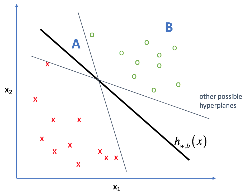
In other words, we'd like to construct a hyperplane that is consistent with the data while committing the least amount to the specific training dataset - models that depend too much on the training data are prone to overfitting. We want to have the most space possible between the decision boundary and the data points on each side of the line in order to increase the total confidence in our predictions.
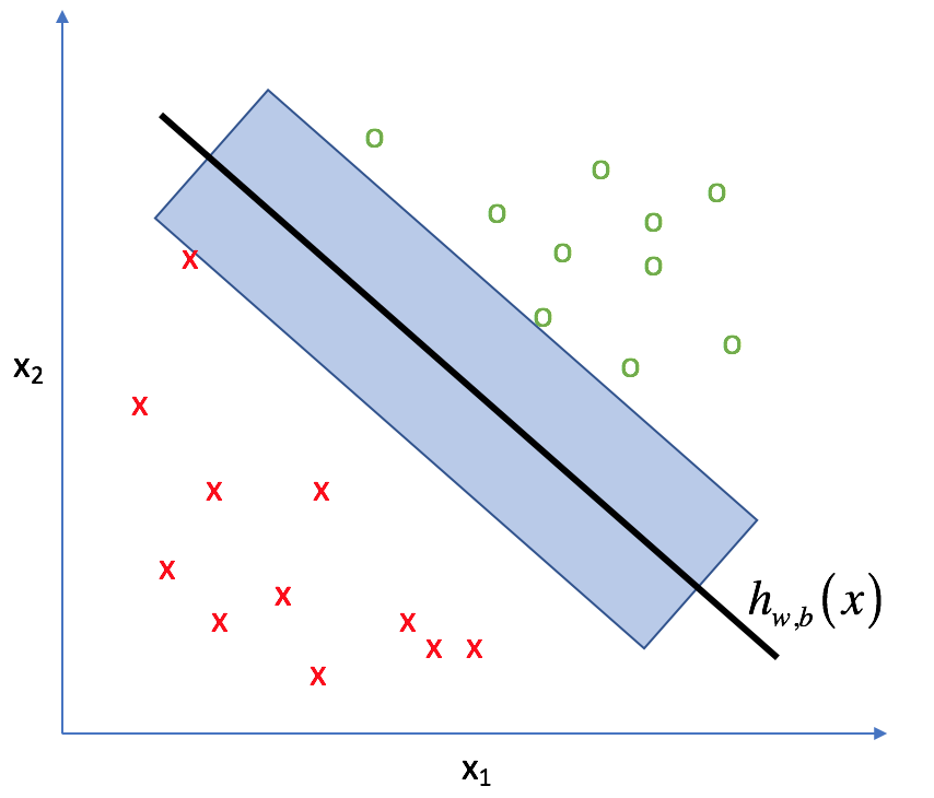
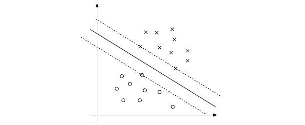
In the world of SVMs, this "space" is called the margin (as visualized below). By maximizing the size of this margin, we can build an optimal classifier.
In practice, there two main ways to measure this margin: the functional margin and the geometric margin.
Functional margin
We can calculate the margin of our hyperplane by comparing the classifier's prediction (${{w^T}x + b}$) to the actual class ($y _i$) since our training dataset has a labeled class for each data point. The functional margin is defined as:
[{{\hat \gamma } _i} = {y _i}\left( {{w^T}x + b} \right)]
When $y _i =1$, we would need a large positive number for ${{w ^T}x + b}$ in order to have a large functional margin, while if $y _i =-1$ we would need a large negative number for ${{w ^T}x + b}$ in order to have a large functional margin. Moreover, our classifier performs a correct classification for all values where ${{\hat \gamma } _i}$ is positive.
One way to maximize this functional margin is to arbitrarily scale $w$ and $b$, since classification with $h_{w, b}$ only depends on the sign, not the magnitude, of the returned value. However, this provides little value and is a weakness of functional margins, as we have no useful way to maximize this expression.
Geometric margin
The geometric margin is defined as the distance from a data point to the decision boundary. How might this be defined? Let's look at the data point labeled "A" in the picture below. Our margin, ${{\hat \gamma } _i}$, defines the scalar length from our data point ($x _i$) to the decision boundary while $\frac{w}{{\left| w \right|}}$ represents the unit direction normal to the decision boundary (ie. the direction of the shortest path from A to B). Using vector subtraction we can define point B as:
[{\bf{\mathord{\buildrel{\lower3pt\hbox{$\scriptscriptstyle\rightharpoonup$}}
\over A} }} - {\gamma _i}\left( {\frac{{\mathord{\buildrel{\lower3pt\hbox{$\scriptscriptstyle\rightharpoonup$}}
\over w} }}{{\left| {\mathord{\buildrel{\lower3pt\hbox{$\scriptscriptstyle\rightharpoonup$}}
\over w} } \right|}}} \right)]
Or in other words:
[{\bf{\mathord{\buildrel{\lower3pt\hbox{$\scriptscriptstyle\rightharpoonup$}}
\over A} }} - {\rm{margin}} = {\bf{\mathord{\buildrel{\lower3pt\hbox{$\scriptscriptstyle\rightharpoonup$}}
\over B} }}]
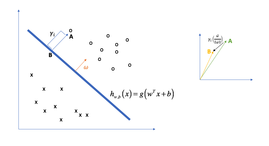
Again, ${\hat \gamma} _i$ is a scalar distance multiplied by a unit vector in the direction perpendicular to the decision boundary, $\frac{w}{{\left| w \right|}}$. As a reminder, the decision boundary is the crossover from where points as classified as 1 or -1, so all values that lie on the decision boundary satisfy the equation ${\omega ^T}x + b = 0$.
Thus, point B in the figure above must satisfy
[{{w^T}{x _B} + b = 0}]
since it lies on the decision boundary. Further, we know that we can calculate $x _B$ as
[{{x _B} = {x^i} - {\gamma _i}\left( {\frac{{\mathord{\buildrel{\lower3pt\hbox{$\scriptscriptstyle\rightharpoonup$}}
\over w} }}{{\left| {\mathord{\buildrel{\lower3pt\hbox{$\scriptscriptstyle\rightharpoonup$}}
\over w} } \right|}}} \right)}]
which, combined with the first equation yields
[{{w^T}\left( {{x^i} - {\gamma _i}\left( {\frac{w}{{\left| w \right|}}} \right)} \right) + b = 0}]
Simplifying this expression, we can solve for an equation that represents our geometric margin, ${\gamma _i}$.
[{{\gamma _i} = \frac{{{w^T}{x^i} + b}}{{\left| w \right|}} = {{\left( {\frac{w}{{\left| w \right|}}} \right)}^T}{x^i} + \frac{b}{{\left| w \right|}}}]
Lastly, we make one small adjustment to keep the margin as a positive number when dealing with both classes ($y=1$ and $y=-1$).
[{\gamma_i} = {y_i}\left( {{{\left( {\frac{w}{{\left| w \right|}}} \right)}^{\text{T}}}{x_i} + \frac{b}{{\left| w \right|}}} \right)]
Notice how the geometric margin is essentially the same thing as the functional margin, except $w$ and $b$ are scaled by a factor of $\frac{1}{{\left| w \right|}}$.
The margin of a hyperplane is formally defined as the smallest calculated margin of all the data points.
[\gamma = \mathop {\min }\limits_{i = 1,...,m} {\gamma_i}]
Summary: The functional margin represents the lowest relative "confidence" of all classified points, while the geometric margin represents the smallest distance from $x_i$ to the hyperplane.
Functional margin:
[{{\hat \gamma }_ i} = {y_i}\left( {{w^T}x + b} \right)]
Geometric margin:
[{\gamma_i} = {y_i}\left( {{{\left( {\frac{w}{{\left| w \right|}}} \right)}^{\text{T}}}{x_i} + \frac{b}{{\left| w \right|}}} \right)]
Note: If ${\left| w \right|}=1$, then the functional margin, ${\hat \gamma }$, and the geometric margin, $\gamma$, are equivalent expressions.
Now that we've sufficiently defined the "space" between our data and the hyperplane, we can now pose an optimization problem to maximize this space.
Parameter optimizations
The following section will present a path towards developing the optimization problem actually used for support vector machines. If the first two approaches are confusing, just skip them.
Approach: directly maximize geometric margin.
The straight-forward approach towards finding the parameters for a hyperplane with the most space between the data and the corresponding decision boundary is to simply maximize the geometric margin. Recall, directly maximizing the functional margin would not be useful as the parameters may be arbitrarily scaled to maximize the resulting margin. However, since the geometric margin is normalized by $\left| w \right|$, scaling $w$ and $b$ have no effect on the resulting margin.
[{\max _{\gamma ,w,b}}\gamma ]
subject to ${y _i}\left( {{w^T}{x _i} + b} \right) \ge \gamma $ for $i = 1,...,m$ and $\left| w \right| = 1{\rm{ }}$.
The first constraint ensures that the maximized margin can be no larger than the smallest distance from an observation to the decision boundary. In essence, this enforces our definition that the geometric margin is $\gamma = \mathop {\min }\limits_{i = 1,...,m} {\gamma _i}$.
Moreover, this optimization favors correct predictions. Recall that any correct prediction will have a value ${y _i}\left( {{w^T}{x _i} + b} \right) > 0$. Thus, by maximizing $\gamma$ subject to ${y _i}\left( {{w^T}{x _i} + b} \right) \ge \gamma$ we are also stating that the want both the most correct predictions and the largest space possible between the decision boundary and our data. Another way to think about this is that a negative margin signifies an incorrect classification and represents the distance a datapoint has "overstepped his bounds".
The second constraint results in a situation where the geometric margin is equal to the functional margin.
Unfortunately, this optimization problem is very difficult to solve computationally, mainly due to its non-convex space.
Approach: rewrite objective in terms of functional margin scaled by ${\left| w \right|}$.
We can express the geometrical margin in terms of the functional margin as $\gamma = \frac{{\hat \gamma }}{{\left| w \right|}}$. Thus, we can rewrite the same objective function as above in terms of the functional margin.
[{\max _{\hat \gamma ,w,b}}\frac{{\hat \gamma }}{{\left| w \right|}}]
subject to ${y _i}\left( {{w^T}{x _i} + b} \right) \ge \hat \gamma $ for $i = 1,...,m$.
Unfortunately, this is still a difficult problem to solve computationally. However, it provides us a clue with what to do instead. Recall that $\hat \gamma$ may be arbitrarily scaled by parameters $w$ and $b$. We can introduce a scaling constraint $\hat \gamma = 1$ without changing the end result. Now you can see that what we are really trying to do is maximize $\frac{1}{{\left| w \right|}}$. Unfortunately, this optimization problem is still difficult to solve.
However, another way to maximize the fraction is to minimize the denominator, which is what we'll do now.
Approach: Focus on minimizing ${\left| w \right|}$.
It turns out that it is much easier to solve the following optimization problem.
[{\min _{\gamma ,w,b}}\frac{1}{2}{\left| w \right|^2}]
subject to ${y _i}\left( {{w^T}{x _i} + b} \right) \ge 1 $ for $i = 1,...,m$.
This is known as a quadratic programming problem which is relatively straight-forward to calculate computationally.
We won't go too much into solving the optimization using quadratic programming, you can simply use a library that has this functionality already built-in, but we will examine it from a high level for a moment.
For the quadratic programming problem, we represent the above optimization as
[{\max _{\alpha ,x,y}}\sum\limits _i {{\alpha _i}} - \frac{1}{2}\sum\limits _{i,j} {{\alpha _i}{\alpha _j}} {y _i}{y _j}x _i^T{x _j}]
subject to ${\alpha _i} \ge 0$ and $\sum\limits _i {{\alpha _i}{y _i} = 0}$ where $i$ and $j$ represent a pair of observations present in the dataset.
In solving this problem, we find a corresponding $\alpha$ value for each observation, $x _i$, in our training dataset.
This $\alpha$ value will then be used to calculate the $w$ vector using the following equation:
[w = \sum\limits _i {{\alpha _i}{y _i}{x _i}} ]
$b$ can also be recovered after $w$ has been solved for.
It turns out that most of the values for $\alpha _i$ will be zero, which effectively nullifies any effect of the corresponding observation, $x _i$, on optimizing our decision boundary. In other words, there are only a select few observations (namely, those close to the decision boundary) which are used in finding the optimal decision boundary. Remember, each observation is a $n$-dimensional vector containing the feature values associated with it. The vectors which correspond with non-zero $\alpha$'s provide all of the necessary support in finding the optimal values for $w$. Hence, the name for our algorithm - support vector machines.
Nonlinear decision boundaries - the kernel trick
The other key part I want to examine in this quadratic programming problem is the term $\sum\limits _{i,j} {{\alpha _i}{\alpha _j}} {y _i}{y _j}x _i^T{x _j}$. Let's break it down.
- ${{\alpha _i}{\alpha _j}}$ determines whether or not this pair of observations is relevant in defining the decision boundary (ie. these values are non-zero).
- ${y _i}{y _j}$ compares the output label of each observation, $x _i$ and $x _j$. This product will be positive if $x _i$ and $x _j$ belong to the same class and negative if $x _i$ and $x _j$ do not belong to the same class.
- $x _i^T{x _j}$ is essentially a representation of how similar the two vectors $x _i$ and $x _j$ are to one another. In this case, we're using the inner product to judge similarity.
With respect to the last term, $x _i^T{x _j}$, if the only thing that matters is the similarity between the two observations, then technically we could modify the actual expression as long as it's still representing "the similarity between vectors $x _i$ and $x _j$."
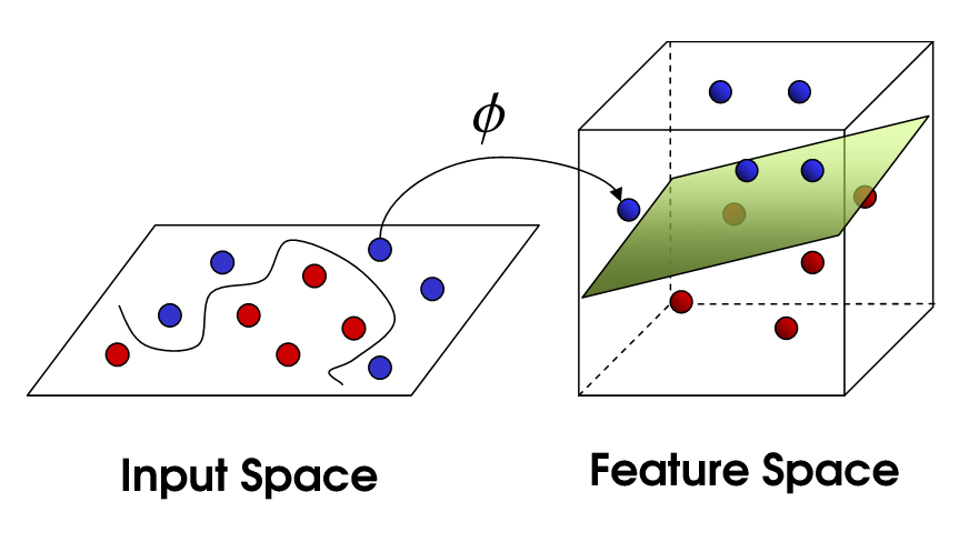
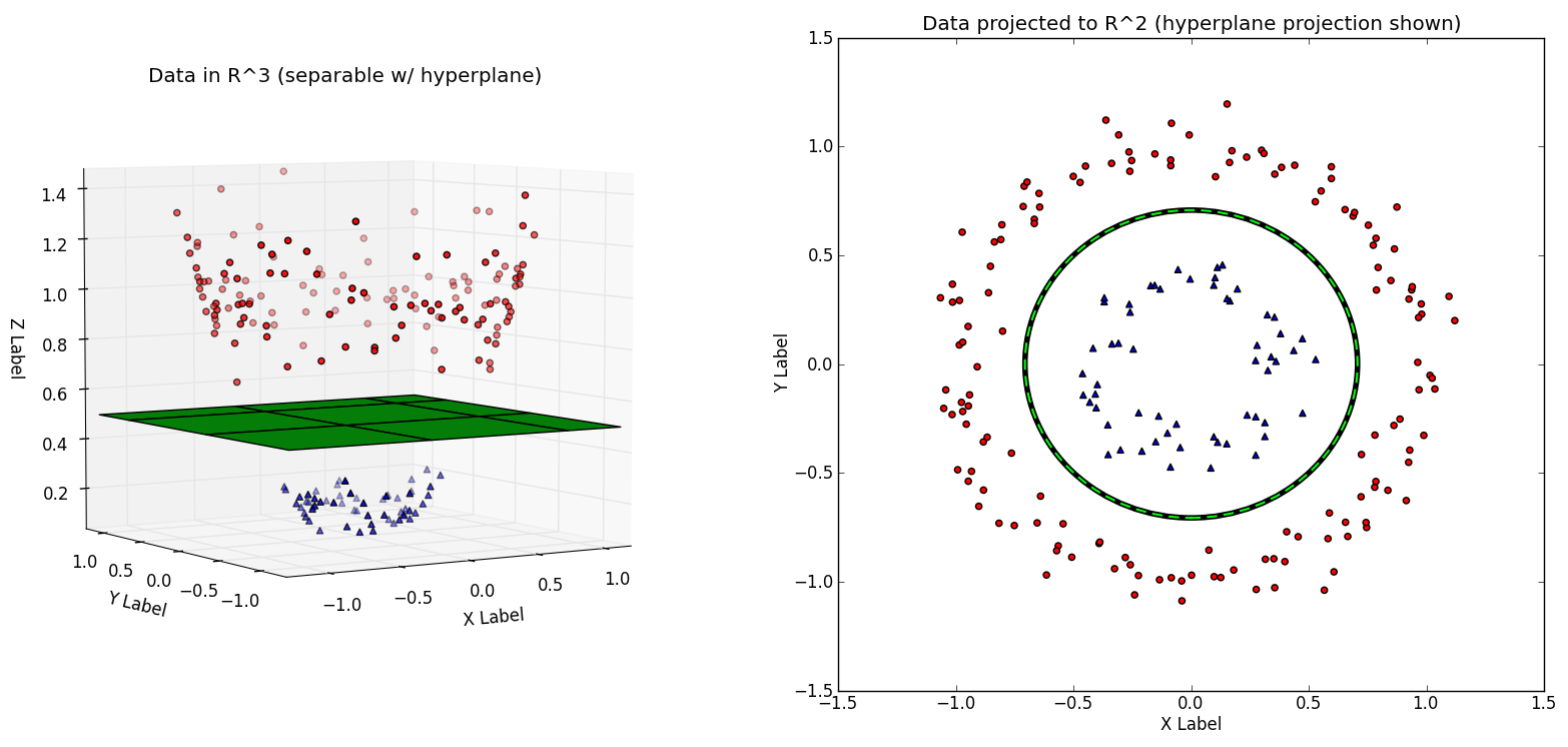
Suppose instead of directly using the vectors $x _i$ and $x _j$, we wished to engineer additional features from the original values using $\phi \left( x \right)$.
We could replace $x _i^T{x _j}$ with $\phi {\left( x \right)^T}\phi \left( z \right)$, which would allow us to more easily find higher-dimensional relationships in the data present.
This new expression is referred to as a kernel.
[K\left( {x,z} \right) = \phi {\left( x \right)^T}\phi \left( z \right)]
However, simply mapping features into higher dimensional space isn't all that impressive. After all, it can be very computationally expensive to perform such high-dimensional calculations. Kernel functions are special in that they operate in a high-dimensional, implicit feature space without ever computing the coordinates of the data in that space.
It can be very expensive to calculate $\phi \left( x \right)$, $\phi \left( z \right)$, and their corresponding dot product. However, the kernel function allows us a method for calculating $K\left( {x,z} \right)$ directly.
By using Kernel functions to create new features, we can transform our classification problem into a higher-dimensional space, draw a linear decision boundary, and then project it back down into the real feature-space resulting in a nonlinear boundary.
Common kernel functions include:
- Linear: $\langle x, x'\rangle$
- Polynomial: $(\gamma \langle x, x'\rangle + r)^d$
- rbf: $\exp(-\gamma |x-x'|^2)$ where $\gamma$ must be greater than 0.
- Sigmoid $(\tanh(\gamma \langle x,x'\rangle + r))$
Regularization
When building an SVM in practice, one of the most common parameters you'll tune is $C$. I'd like to take just a brief moment to examine this.
We can reformulate our optimization objective to include a regularization term, a common technique to prevent overfitting.
Our new optimization problem is as follows:
[{\min _{\gamma ,w,b}}\frac{1}{2}{\left| w \right|^2} + C\sum\limits _{i = 1}^m {{\xi _i}} ]
such that ${y _i}\left( {{w^T}{x _i} + b} \right) \ge 1 - {\xi _i}$ for $i = 1,...,m$ and ${\xi _i} \ge 0$ for $i = 1,...,m$.
Essentially, we are now allowing the decision boundary to do a worse job classifying a few points in favor of doing a better job on the majority. Focusing on the majority allows for us to build a model which is more likely to generalize well and prevents our decision boundary from fluctuating wildly if we start to introduce outliers when training.
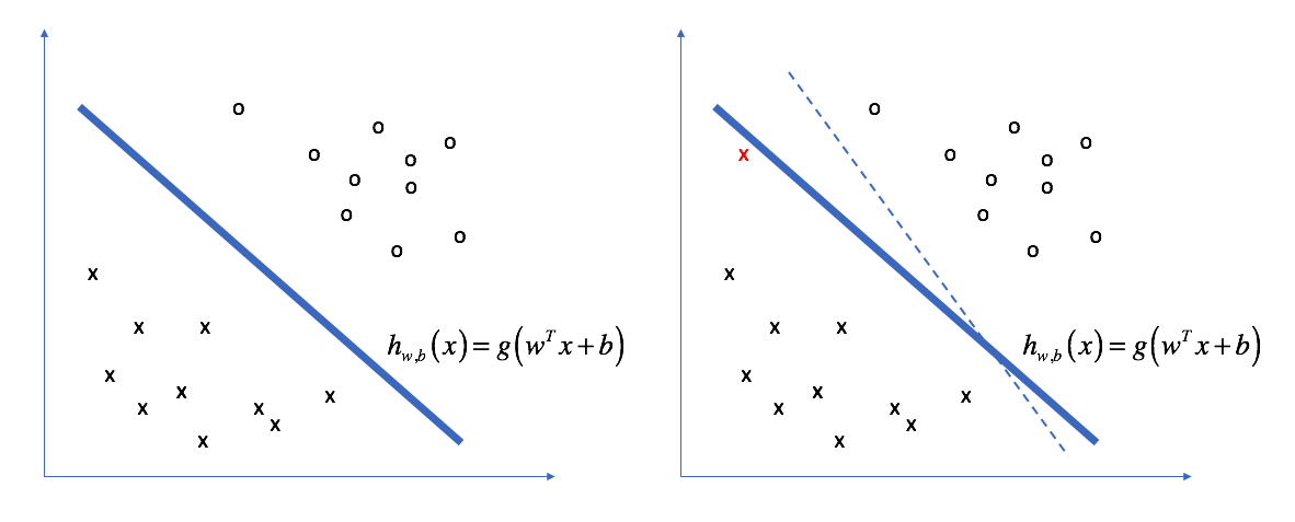
Hence, $C$ controls the tradeoff between the smoothness of a decision boundary and accuracy of correct classifications.
Further reading
Support Vector Machines - CS229 Lecture notes - Andrew Ng
Support Vector Machine (SVM) Tutorial