K-nearest neighbors.

Many machine learning techniques involve building a model that is capable of representing the data and then finding the optimal parameters for the model to minimize error. K-nearest neighbors, however, is an example of instance-based learning where we instead simply store the training data and use it to make new predictions.
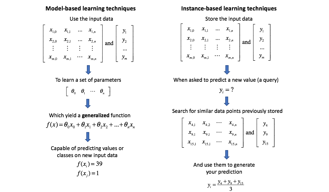
In general, instance-based techniques such as k-nearest neighbors are lazy learners, as compared to model-based techniques which are eager learners. A lazy approach will only "learn" from the data (to make a prediction) when a new query is made while an eager learner will learn from the data right away and build a generalized model capable of predicting any value. Thus, lazy learners are fast to train and slower to query, while eager learners are slower to train but can make new predictions very quickly.
K-nearest neighbors is based on the assumption of locality in your data, that nearby points have similar values. Thus, what's a good way to predict a new data point? Just look for similar observations in your training data and develop your best guess. More specifically, use the k-nearest observations to formulate your prediction. For regression, this prediction is some measure of the average value (ie. mean) of the surrounding neighbors. For classification, this prediction is a result of some voting mechanism (ie. mode) of the surrounding neighbors.
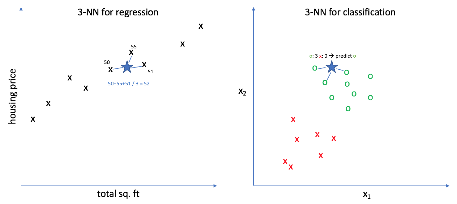
In the example above, we selected $k=3$ to show an example of k-nearest neighbors for both regression and classification.
Finding similar observations (measures of distance)
In order to find the k-nearest neighbors, we must first define some measure of "closeness" (in order words, distance). Remember, our observations exist within an n-dimensional featurespace; as it turns out, there are many ways to measure the distance between two points in space.
In sklearn's implementation for k-nearest neighbors, you can use any of the available methods found in the DistanceMetric class. Remember, we're using distance as a proxy for measuring similarity between points.
One important note to make is that since we're using distance as a measure of similarity, we're implicitly constraining our model to weight all features equally; distance in the $x _1$ dimension is on the same scale as distance in the $x _n$ dimension. The best way to deal with data containing features of varying importance is to simply feed the KNN algorithm more data; given sufficient training data (sometimes this might mean hundreds of thousands of examples), the detrimental effect of implicitly weighting all features equally will diminish.
Choosing k
After selecting a metric to be used for finding the observations closest to the query, you must determine how many of the nearest neighbors you'd like to take into account. By default, sklearn.neighbors.KNeighborsRegressor and sklearn.neighbors.KNeighborsClassifier use 5 as the default value for n_neighbors (otherwise known as $k$), but this can easily be optimized using something like K-fold cross validation to try out different values for $k$ and determine the best choice. A common rule of thumb seems to be that $\sqrt n$, where $n$ is the number of samples in your training set, seems to often perform well.
Consider the case where we set $k=n$. Wherever our query point is, we'd end up using the entire dataset to predict the value. If we're using a simple average, the resulting predictor will return a constant value regardless of the input features. For classification, you'll always end up classifying new data points as whichever class is most prevalent in the training dataset. For regression, you'll always end up return the mean value of the entire training dataset. However, if we instead use a weighted average for prediction, where data points closer to the query take on higher weights, how would the results look? Let's take a dive into a Jupyter notebook and explore this.
First, let's load an example dataset and prepare the data for training and testing.
from sklearn.datasets import load_boston
from sklearn.model_selection import train_test_split

boston = load_boston()
features_train, features_test, labels_train, labels_test = train_test_split(boston.data, boston.target,
                                                                            test_size=0.4, random_state=0)

import pandas as pd

features_train = pd.DataFrame(features_train, columns = boston.feature_names)
features_test = pd.DataFrame(features_test, columns = boston.feature_names)
# Select rooms column for univariate regression example
features_train = features_train.iloc[:, 5]
features_test = features_test.iloc[:, 5]

labels_train = pd.DataFrame(labels_train, columns = ['Price'])
labels_test = pd.DataFrame(labels_test, columns = ['Price'])
Next, I'll just take a peek at the data to see what we're working with.
import matplotlib.pyplot as plt
%matplotlib inline

plt.scatter(features_train, labels_train)
Lastly, I'll train six KNN models with varying weights and values for $k$.
from sklearn.neighbors import KNeighborsRegressor
import numpy as np

n = features_train.shape[0]
params = [{'weights': 'uniform', 'n_neighbors': 3},
          {'weights': 'distance', 'n_neighbors': 3},
          {'weights': 'uniform', 'n_neighbors': np.sqrt(n).astype(int)},
          {'weights': 'distance', 'n_neighbors': np.sqrt(n).astype(int)},
          {'weights': 'uniform', 'n_neighbors': n},
          {'weights': 'distance', 'n_neighbors': n}]

plot_range = np.arange(min(features_train), max(features_train), 0.01)

for i, param in enumerate(params):
    model = KNeighborsRegressor(**params[i])
    model.fit(features_train.values.reshape(-1, 1), labels_train)

    pred = model.predict(plot_range.reshape(-1, 1))
    # Sort values for plotting
    new_X, new_y = zip(*sorted(zip(plot_range.reshape(-1, 1), pred)))
    plt.subplot(3, 2, i + 1)
    plt.scatter(features_train.values.reshape(-1, 1), labels_train, c='k', label='data')
    plt.plot(new_X, new_y, c='g', label='prediction')
    plt.legend()
    plt.title("KNeighborsRegressor (k = %i, weights = '%s')" % (params[i]['n_neighbors'], params[i]['weights']))
    plt.ylabel('Price')
    plt.xlabel('Number of rooms')

plt.rcParams["figure.figsize"] = [24, 14]

plt.show()
The result is shown below.
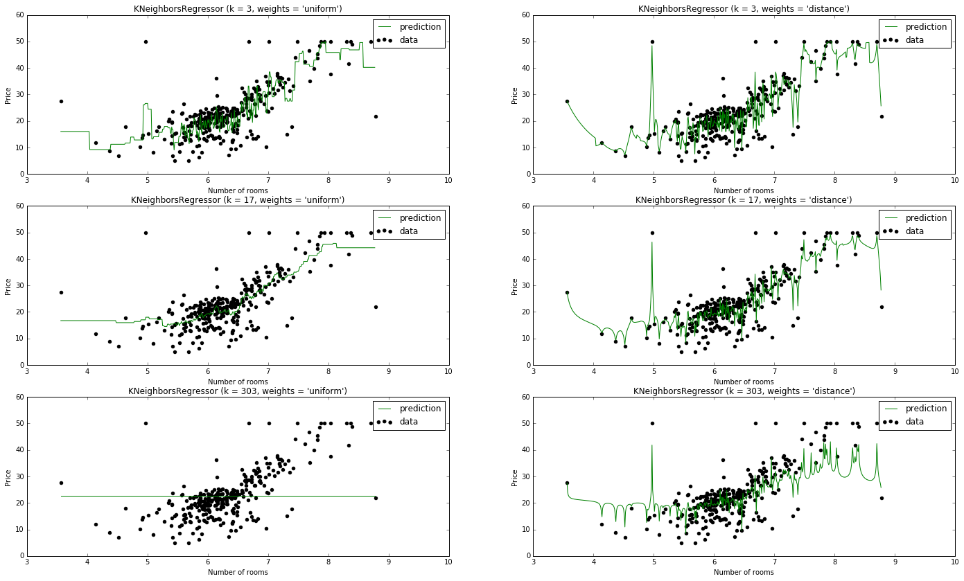
I kind of jumped ahead of myself, as we haven't finished discussing the considerations of the KNN algorithm, but I wanted to go ahead and show you the effect of $k$.
Note: The rule of thumb $k = \sqrt n$ seems to be our best model.
Tying things together (selecting neighbors)
Now that we've established a metric for measuring similarity and picked how many neighbors we'd like to include in the prediction, we need a method to search through our stored data to find the k-nearest neighbors. A brute force search, simply calculating the distance of our query from every point in our dataset, will work fairly well with small datasets but becomes undesirably slow at larger scales. Tree-based approaches can bring greater efficiencies to the search process by inferring distances. For example, if $A$ is very far from $B$ and $C$ is very close to $B$, we can infer that $A$ is also far from $C$ without explicitly measuring the distance. The sklearn documentation covers the K-D Tree and Ball Tree search algorithms, as well as some practical advice on choosing a specific search algorithm.
Using stored data for predictions (measures of the average)
After we've found the k-nearest neighbors, we can use their information to predict a value for the query.
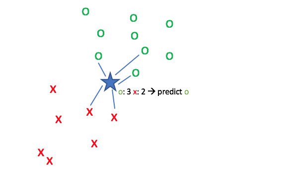
Classification
So you have a new observation with features $x _i$ and you'd like to predict the class label, $y _i$. You've queried the KNeighborsClassifier and found the $k$ nearest neighbors. Now you're tasked with using the information present among the $k$ neighbors to predict $y _i$.
The simplest method is to conduct a uniform vote where each neighbor essentially casts one vote to say "the query shares the same class as me". In the event that your vote ends in a tie, choose the label which is more common across the entire dataset.
However, we can perform a more accurate vote if we decide to weight each vote based on how close it is to the query point. This is accomplished by weighting each vote by the inverse of its distance from the query so that closer points have stronger votes.

Regression
Now let's suppose you have a new observation with features $x _i$ and you'd like to predict a continuous target output, $y _i$. You've queried the KNeighborsRegressor and found the $k$ nearest neighbors. Now you're tasked with using the information present among the $k$ neighbors to predict $y _i$.
The approach is largely the same as discussed above for classifiers, but rather than establishing a voting mechanism we'll simply calculate the mean of the neighbor's $y$ values. We can still use uniform or distance weighting.
Fun fact: You can combine k-nearest neighbors with linear regression to build a collection of linear models as a predictor. Read more here.
Summary
K-nearest neighbors is an example of instance-based learning where we store the training data and use it directly to generate a prediction, rather than attempted to build a generalized model.
The three main things you must define for a KNN algorithm is a way to measure distance, how many neighbors ($k$) to use in your predictions, and how to average the information from your neighbors to generate a prediction.