Linear regression.

Linear regression is used to predict an outcome given some input value(s). While machine learning classifiers use features to predict a discrete label for a given instance or example, machine learning regressors have the ability use features to predict a continuous outcome for a given instance or example. For example, a classifier might draw a decision boundary that can tell you whether or not a house is likely to sell at a given price (when provided with features of the house) but a regressor can use those same features to predict the market value of the house. Nonetheless, regression is still a supervised learning technique and you'll still need to train your model on a set of examples with known outcomes.
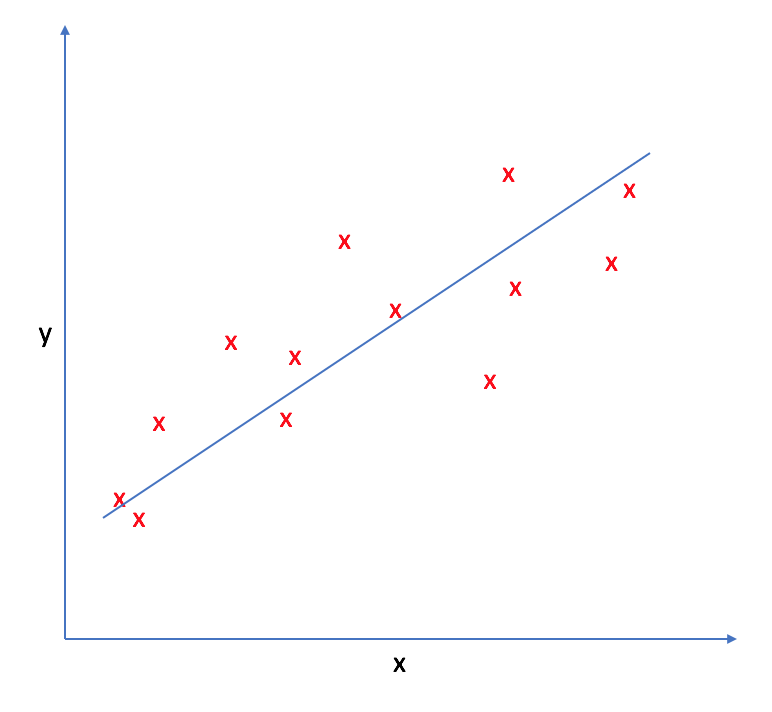
The basic premise behind linear regression is to provide a model which can observe linear trends in the data; you've probably encountered linear regression at some point in the past as finding the "line of best fit".
The model
Our machine learning model is represented by the equation of a line.
$${h_\theta }\left( x \right) = {\theta _0} + {\theta _1}x$$
In this case, we define our model as ${h _\theta }\left( x \right)$ where $h$ represents our predicted outcome as a function of our features, $x$. Typically, the model of a line is represented by $y=mx+b$. We use $h$ instead of $y$ to denote that this model is a hypothesis of the true trend. In a sense, we're attempting to provide our "best guess" for finding a relationship in the data provided. $\theta _0$ and $\theta _1$ are coefficients of our linear equation (analogous to $b$ and $m$ in the standard line equation) and will be considered parameters of the model.
So far, our model has only been capable of capturing one independent variable and mapping its relationship to one dependent variable. We'll now extend our linear model to allow for $n$ different independent variables (in our case, features) to predict one dependent variable (an outcome).
Thus, for each input $x$ we'll have a vector of values
each with corresponding coefficients, $\theta$.
Note: $x _0 = 1$ by convention. This allows us to do matrix operations with $x$ and $\theta$ without deviating from our defined linear model.
Extending this model to account for multiple inputs, we can write it as
$${h _\theta }\left( x \right) = {\theta _0} + {\theta _1}{x _1} + {\theta _2}{x _2} + {\theta _3}{x _3} + ... + {\theta _n}{x _n}$$
or more succinctly as
$${h_\theta }\left( x \right) = {\theta ^T}x$$
when dealing with one example or
$${h _\theta }\left( x \right) = X\theta $$
when dealing with $i$ examples.
Note: this matrix, $X$, is also referred to as the design matrix and is usually capitalized by convention to denote it as a matrix as opposed to a vector.
If that doesn't quite make sense, let's take a step back and walk through the representation.
For a univariate model, we could write the model in matrix form as:
Go ahead and do the matrix multiplication to convince yourself.
Now that you're convinced, let's extend this to a multivariate model with $j$ features and $i$ examples.
This is pretty useful because we can go ahead and calculate the prediction, ${{h _\theta }\left( {{x _i}} \right)}$, for every example in our data set using one matrix operation.
The cost function
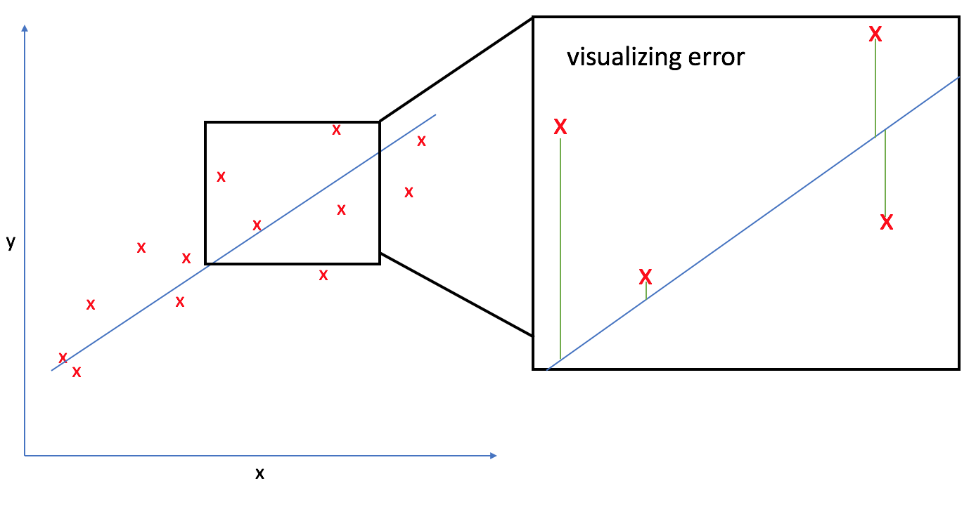
In order to find the optimal line to represent our data, we need to develop a cost function which favors model parameters that lead to a better fit. This cost function will approximate the error found in our model, which we can then use to optimize our parameters, $\theta _0$ and $\theta _1$, by minimizing the cost function. For linear regression, we'll use the mean squared error - the average difference between our guess, ${{h _\theta }\left( {{x _i}} \right)}$, and the true value, ${{y _i}}$ - to measure performance.
$$\min \frac{1}{{2m}}\sum\limits_{i = 1}^m {{{\left( {{h _\theta }\left( {{x _i}} \right) - {y _i}} \right)}^2}} $$
Substituting in our definition of the model, ${{h _\theta }\left( {{x _i}} \right)}$, we'll update our cost function as:
$$J\left( \theta \right) = \frac{1}{{2m}}\sum\limits _{i = 1}^m {{{\left( {\left( {\sum\limits _{j = 0}^n {{\theta _j}{x _{i,j}}} } \right) - {y _i}} \right)}^2}}$$
Finding the best parameters
There's a number of ways to find the optimal model parameters. A few common approaches are detailed below.
Gradient descent
We use gradient descent to perform the parameter optimization in accordance with our cost function. Remember, the cost function essentially will score how well our model is fitting the present data. A smaller cost function means less error, which means we have a better model.
We first start with an initial guess for what our parameter values should be. Gradient descent will then guide us through an iterative process of updating our parameter weights in search of an optimum solution.
Let's first look at the simplest example, where we fix $\theta _0 = 0$ and find the optimal slope value.
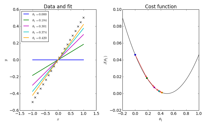
Using gradient descent, the weights will continue to update until we've converged on the optimal value. For linear regression, the cost function is always convex with only one optimum, so we can be confident that our solution is the best possible one. This is not always the case, and we'll need to be weary of converging on local optima using other cost functions.
As the picture depicts, gradient descent is an iterative process which guides the parameter values towards the global minimum of our cost function.
$${\theta _j}: = {\theta _j} - \eta \frac{\partial }{{\partial {\theta _j}}}J({\theta _0},{\theta _1})$$
Gradient descent will update your parameter value by subtracting the current value by the slope of the cost function at that point multiplied by a learning rate, which basically dictates how far to step. The learning rate, $\eta$, is always positive.
Notice in the picture above how the first attempted value, $\theta _1 = 0$, has a negative slope on the cost function. Thus, we would update the current value by subtracting a negative number (in other words, addition) multiplied by the learning rate. In fact, every point left of the global minimum has a negative slope and would thus result in increasing our parameter weight. On the flip side, every value to the right of the global minimum has a positive slope and would thus result in decreasing our parameter weight until convergence.
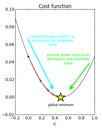
One neat thing about this process is that gradient descent will automatically slow down as we're nearing the optimum. See how the initial iterations take relatively large steps in comparison to the last steps? This is because our slope begins to level off as we approach the optimum, resulting in smaller update steps. Because of this, there is no need to adjust $\eta$ during the optimization.
We can extend this idea to update both $\theta _0$ and $\theta _1$ simultaneously. In this case, our 2D curve has become a 3D contour plot.
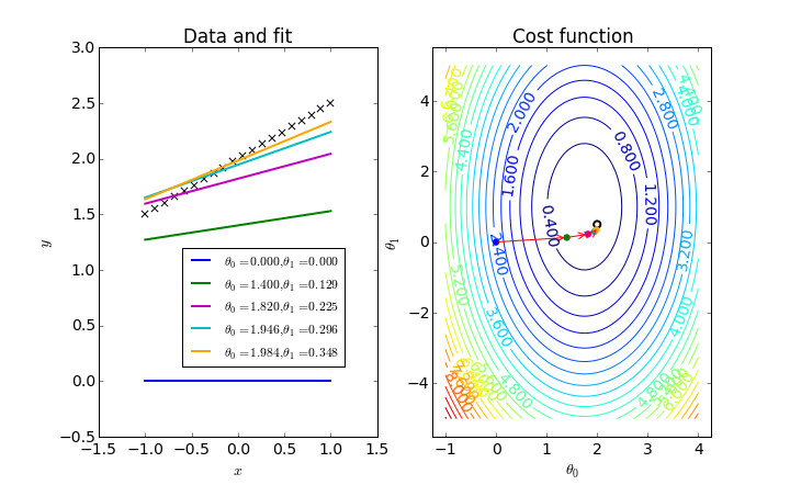
While the gradient descent algorithm remains largely the same,
$${\theta _j}: = {\theta _j} - \alpha \frac{\partial }{{\partial {\theta _j}}}J\left( \theta \right)$$
we now define the differential as
$$\frac{\partial }{{\partial {\theta _j}}}J\left( \theta \right) = \frac{1}{m}\sum\limits _{i = 1}^m {\left( {\left( {\sum\limits _{j = 0}^n {{\theta _j}{x _{i,j}}} } \right) - {y _i}} \right)} {x _{i,j}}$$
using the chain rule.
A few notes and practical tips on this process.
- Scaling your features (as mentioned in Preparing data for a machine learning model) to be on a similar scale can greatly improve the time it takes for your gradient descent algorithm to converge.
- It's important that your learning rate is reasonable. If it is too large it may overstep the global optimum and never converge, and if it's too small it will take a very long time to converge.
- Plot the $J\left( \theta \right)$ as a function of the number of iterations you have run gradient descent. If gradient descent is working properly it will continue to decrease steadily until leveling off, hopefully, close to zero. You can also use this plot to visually determine when your cost function has converged and gradient descent may be stopped.
- If $J\left( \theta \right)$ begins to increase as the number of iterations increases, something has gone wrong in your optimization. Typically, if this occurs it is a sign that your learning rate is too large.
Gradient descent is often the preferred method of parameter optimization for models which have a large number (think, over 10,000) of features.
Normal equation
Remember how we used matrices to represent our model? Using normal equation for linear regression you can solve for the optimal parameters analytically in one step.
$$\theta = {\left( {{X^T}X} \right)^{ - 1}}{X^T}y$$
You can find a good derivation for this equation here.
The benefit of using the normal equation to solve for our model parameters is that feature scaling is not necessary and it can be more effective than gradient descent for small feature sets.
A few notes and practical tips on this process.
- This method will occasionally give you problems when dealing with noninvertible or degenerate matrices. If this is the case, it is likely that your feature set has redundant (linearly dependent) features, or simply too many features with respect to the number of training examples given.
Implementation
Linear regression is very simple to implement in sklearn. It can accommodate both univariate and multivariate models and will automatically handle one-hot encoded categorical data to avoid the dummy variable trap.
from sklearn.linear_model import LinearRegression
model = LinearRegression()
model.fit(features_train, labels_train)
predictions = model.predict(features_test)

import matplotlib.pyplot as plt

plt.scatter(features, labels, color = 'red')
plt.plot(features_test, predictions, color = 'blue')