Generalizing value functions for large state spaces.

Up until now, we've discussed the concept of a value function primarily as a lookup table. As our agent visits specific state-action pairs and continues to explore an environment, we update the value of that state-action pair independent of any other state-action pairs. When we'd like to know the value, we simply query our lookup table and report the value. However, this makes an incredibly difficult case for learning in environments with large state spaces. For example, the game of Go has $10^{170}$ possible states; it would be impractical to build a lookup table for such an environment - both due to the size required to store such a table and the amount of training required to visit all of the states. Even more challenging, some environments (such as the case for robotics) exist in a continuous state space.
Clearly, a lookup table is not a practical model for representing our value function. Ideally, we'd have a model that can generalize concepts of value across similar states. In order to do this, we'll need to develop a set of features that adequately describe the states in such a manner that we can identify similar states based on their features. In short, we're looking for a more efficient representation of state than simply viewing each one in isolation.
We can then develop a parametric model, such as a linear addition of features or a neural network, which can learn to regress the value of a state given its features. The parameters of this model can be trained to approximate our current estimates for the value of states given our agent's experience.
Function approximation
In earlier posts, we've mainly been focused on estimating the action value function, $Q\left( {S,A} \right)$, given that it allows us to perform model-free learning. Thus, we'll need to develop a feature representation that adequately describes state-action pairs.
${\bf{x}}$ is a vector of length $n$ which contains $n$ features that describe a given state-action pair. These features will be in the input to our value function model. For the simple case of a linear model, the value of a state-action pair will be calculated as
$$ \hat q\left( {S,A} \right) = {x_1}\left( {S,A} \right){\theta_1} + ... + {x_n}\left( {S,A} \right){\theta_n} $$
or more succinctly as
$$ \hat q\left( {S,A,\theta } \right) = {\mathbf{x}}{\left( {S,A} \right)^{\text{T}}}\theta $$
where $\theta$ represents the vector of learned parameters of our function approximator.
There's three main types of value function approximation:
- Given a state, what is the value of that state?
- Given a state and action, what is the value of that state-action pair?
- Given a state, what is the value of all possible actions taken from that state?
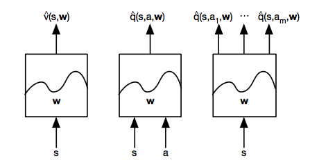
Each of these models are defined by a set of parameters, $\theta$ (also sometimes referred to as weights, $w$). With this value function approximator, we'll input a feature vector that describes a state or state-action pair and output the approximated value. In the following section, I'll discuss how we can train these model parameters to most closely match our best estimate of the value function.
Training the parameters of our value function approximator
Suppose that we had were able to compare the true value of states to our approximated value. If this were the case, we would have a supervised learning environment where we could simply establish a loss function and adjust our parameters to minimize this loss. One popular optimization method is gradient descent, a topic I've covered previously. We can use this algorithm to find a set of parameters which exist at a local minimum of the loss function.
As a reminder, gradient descent allows us to find a local minimum by iteratively adjusting the parameters of a function in the negative direction of the function gradient. The parameter update may be written as
$$ \Delta \theta = - \alpha {\nabla_\theta }J\left( \theta \right) $$
where $\alpha$ denotes the step size for the update.
Let's use mean squared error as a loss function to compare the true value function, ${q_\pi }\left( {S,A} \right)$, and our approximate value function, $\hat q\left( {S,A,\theta } \right)$, characterized by parameters $\theta$. Specifically, we'll define our loss function, $J\left( \theta \right)$ as the expectation of the squared error, where the expectation is the mean value.
$$ J\left( \theta \right) = \mathbb{E}\left[ {{{\left( {{q_\pi }\left( {S,A} \right) - \hat q\left( {S,A,\theta } \right)} \right)}^2}} \right] $$
We can calculate the gradient of our cost function using the chain rule.
$$ {\nabla_\theta }J\left( \theta \right) = -2\left( {{q_\pi }\left( {S,A} \right) - \hat q\left( {S,A,\theta } \right)} \right){\nabla_\theta }\hat q\left( {S,A,\theta } \right) $$
Plugging this in to our gradient descent algorithm, we can find the final rule for our parameter update.
$$ \Delta \theta = \alpha \left( {{q_\pi }\left( {S,A} \right) - \hat q\left( {S,A,\theta } \right)} \right){\nabla_\theta }\hat q\left( {S,A,\theta } \right) $$
Note: the two negative signs canceled out and the constant was absorbed into our step size, $\alpha$.
As an example, let's look at the case where our value function approximator is a linear model.
$$ \hat q\left( {S,A,\theta } \right) = {\mathbf{x}}{\left( {S,A} \right)^{\text{T}}}\theta $$
Thus, our cost function may be written as
$$ J\left( \theta \right) = \mathbb{E}\left[ {{{\left( {{q_\pi }\left( {S,A} \right) - {\mathbf{x}}{{\left( {S,A} \right)}^{\text{T}}}\theta } \right)}^2}} \right] $$
where we've substituted our model in for ${\hat q}$.
The gradient of ${\hat q}$ is simply our feature vector, ${\nabla_\theta }\hat q = {{\mathbf{x}}\left( {S,A} \right)}$. Thus, the update rule for a linear model is simply the product of our step size, prediction error, and feature values.
$$ \Delta \theta = \alpha \left( {{q_\pi }\left( {S,A} \right) - \hat q\left( {S,A,\theta } \right)} \right){\mathbf{x}}\left( {S,A} \right) $$
Updating towards a target
Unfortunately, we can't use the gradient descent equations presented above because reinforcement learning isn't a supervised learning problem; we don't know the true value function. However, we've previously covered methods for estimating the value function such as Monte Carlo learning, temporal difference learning, and a hybrid approach. As a reminder, we can iteratively update our estimate of the value function as our agent explores an environment and gains experience. Thus, we can substitute a target value from one of our value function estimation methods for ${q_\pi }$ in the gradient descent algorithm described previously.
- For Monte Carlo learning, the target is the return, $G_t$.
$$ \Delta {\theta ^{MC}} = \alpha \left( {{G_t} - \hat q\left( {S,A,\theta } \right)} \right){\nabla_\theta }\hat q\left( {S,A,\theta } \right) $$
The return, $G_t$, represents the future sequence of rewards observed after an agent visited a state-action pair. This is an unbiased, albeit noisy, sample of the true value. Given data for an episode
$$ \left\langle {\left( {{S_1},{A_1}} \right),{G_1}} \right\rangle ,\left\langle {\left( {{S_2},{A_2}} \right),{G_2}} \right\rangle ,...,\left\langle {\left( {{S_T},{A_T}} \right),{G_T}} \right\rangle $$
we can apply supervised learning to fit a model which maps the features describing a state-action pair to the resulting return.
- For $TD\left( 0 \right)$ learning, the target is ${{R_{t}} + \gamma \hat q\left( {S_{t+1},A_{t+1},\theta } \right)}$.
$$ \Delta {\theta ^{TD\left( 0 \right)}} = \alpha \left( {\left( {{R_{t}} + \gamma \hat q\left( {S_{t+1},A_{t+1},\theta } \right)} \right) - \hat q\left( {S,A,\theta } \right)} \right){\nabla_\theta }\hat q\left( {S,A,\theta } \right) $$
The target, ${{R_{t}} + \gamma \hat q\left( {S_{t+1},A_{t+1},\theta } \right)}$, is a biased sample of the true value. Given set of training data
$$ \left\langle {\left( {{S_1},{A_1}} \right),{R_1} + \gamma Q\left( {{S_2},{A_2},\theta } \right)} \right\rangle ,\left\langle {\left( {{S_2},{A_2}} \right),{R_2} + \gamma Q\left( {{S_3},{A_3},\theta } \right)} \right\rangle ,...,\left\langle {\left( {{S_T},{A_T}} \right),{R_T}} \right\rangle $$
we can similarly fit a model which maps the features describing a state-action pair to the resulting TD target.
- For $TD\left( \lambda \right)$ learning, we discussed targets for both a forward-view and backward-view perspective.
The forward-view target, ${q_t^\lambda }$, is simply the weighted sum of all $n$-step returns for values of $n$ ranging from $n=1,...,T$ where $T$ signifies the terminal state.
$$ \Delta {\theta ^{TD\left( \lambda \right)}} = \alpha \left( {q_t^\lambda - \hat q\left( {S,A,\theta } \right)} \right){\nabla_\theta }\hat q\left( {S,A,\theta } \right) $$
The backward-view target combines a TD error, $\delta_t$, with the elibility of state-action pairs to be updated. However, we now define our eligilibity trace in terms of our features (by looking at ${\nabla_\theta }\hat q$) rather than storing an eligibility for each individual state-action pair.
$$ {\delta_t} = {R_t} + \gamma \hat q\left( {{S_{t + 1}},{A_{t + 1}},\theta } \right) - \hat q\left( {{S_t},{A_t},\theta } \right) $$
$$ {E_t} = \gamma \lambda {E_{t - 1}} + {\nabla_\theta }\hat q\left( {{S_t},{A_t},\theta } \right) $$
$$ \Delta {\theta ^{TD\left( \lambda \right)}} = \alpha {\delta_t}{E_t} $$
Incremental updates
We can use stochastic gradient descent, an online optimization technique that updates parameters on a single observation, to train the model parameters at each step as our agent explores the environment. Essentially, we'll use our model to predict the value of taking some action in a given state, proceed to take that action and build a more informed estimate of the value of the given state-action pair, and then use gradient descent to update our parameters to minimize that difference. We'll continue to do this following the trajectory of our agent for the duration of the exploration.
Because we're performing a parameter update on single observations, it's somewhat of a noisy (stochastic) optimization process, but it allows us to immediately improve our model after each step of experience and the model eventually converges to a local optimum in most cases. However, this approach often fails to converge when using a non-linear function approximator, such as a neural network.
Batch updates
Although we can reach convergence in some instances of incremental gradient descent updates, it's not a very efficient use of our experiences given that we essentially throw away each transition after updating the parameters. In fact, a better way to leverage this experience is to store it in a dataset, $D$, as a collection of individual transitions $\left( {{s_t},{a_t},{r_t},{s_{t + 1}}} \right)$.
We can then proceed to randomly sample this dataset, referred to as replay memory, performing stochastic gradient descent to optimize the parameters of our value function approximator until we've reached convergence under a process known as experience replay. In essence, we're able to get more out of our data by going over it multiple times (ie. replaying transitions) rather than discarding transitions after only one update.
In an incremental approach, the transitions used to update our parameters are highly correlated and can cause our parameter optimization to blow up (ie. fail to converge). However, with experience replay we randomly sample from a collection of transitions, breaking the correlation between observations that were present along a given trajectory. This has the effect of stabilizing the parameter optimization and yields much better results.
Fixed targets
For targets based on the temporal difference approach, it's important to note that these targets are based on the approximated value function which we are attempting to optimize. To avoid any potential feedback loops that would destabilize training, it's best to optimize the parameters of ${\hat q}$ against a fixed target that uses parameters from some previous point in training. Thus, we'll need to store two sets of parameters: the parameters of the approximated value function after $i$ training iterations, ${\theta_i}$, and the fixed parameters, ${\theta_{fixed}}$, to be used when calculating our target. This set of fixed parameters will be updated periodically during training to improve to accuracy of our targets.
For example, the cost function for a Q-learning algorithm will use the fixed parameters, ${\theta_{fixed}}$, in calculating the target, while optimizing ${\theta_i}$ with gradient descent.
$$ J\left( \theta \right) = {\mathbb{E}_ {{s_t},{a_t},{r_t},{s_{t + 1}}~{D_i}}}\left[ {{{\left( {r + \gamma \mathop {\max Q\left( {s',a',{\theta_{fixed}}} \right) - Q\left( {s,a,{\theta_i}} \right)}\limits_{a'} } \right)}^2}} \right] $$