Learning in a stochastic environment.

Previously, I discussed how we can use the Markov Decision Process for planning in stochastic environments. For the process of planning, we already have an understanding of our environment via access to information given by the transfer function and reward function. In other words, we defined the world and simply wanted to calculate the optimal method of completing some task. For the case of reinforcement learning, our agent will explore and learn about the world as it assumes different states within the environment.
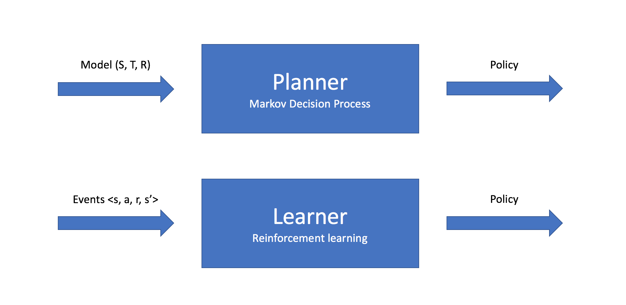
You can think of planning as the process of taking a model (a fully defined state space, transition function, and reward function) as input and outputting a policy on how to act within the environment, whereas reinforcement learning is the process of taking a collection of individual events (a transition from one state to another and the resulting reward) as input and outputting a policy on how to act within the environment. These individual transitions are collected as the agent explores various states within the environment.
Defining the value of an action
Previously, we defined equations to represent the utility and optimal policy for a state.
$$U\left( s \right) = R\left( s \right) + \gamma \mathop {\max }\limits _a \sum\limits _{s'} {T\left( {s,a,s'} \right)} U\left( {s'} \right)$$
$$\pi {\left( s \right)^*} = \arg \mathop {\max }\limits _a \sum\limits _{s'} {T\left( {s,a,s'} \right)} U\left( {s'} \right)$$
Given a specified state, we're evaluating the different actions we could take to proceed into the next state, and choosing the action which yields the greatest benefit (ie. transfers the agent to the most valuable state). Thus, it would make sense to develop an expression which directly represents the value for performing an action in a given state.
Specifically, we'll define a new function, $Q\left( {s,a} \right)$, that evaluates the value of existing in a state, performing an action which transitions us to a new state, and then proceeding to follow some policy thereafter.
Similar to the utility function for states, we can define this as an expectation of accumulated reward - the only difference is that we're now enforcing the agent's first action.
$$ Q\left( {s,a} \right) = E\left[ {\sum\limits_ {t = 0}^\infty {{\gamma ^t}R\left( {{S_ t}} \right)|{S_ 0} = s,{A_ 0} = a} } \right] $$
Next, let's expand this summation.
$$ Q\left( {s,a} \right) = E\left[ {R\left( {{S_ t}} \right) + \gamma R\left( {{S_ {t + 1}}} \right) + {\gamma ^2}R\left( {{S_ {t + 2}}} \right) + ...|{S_ t} = s,{A_ t} = a} \right] $$
Because we've instructed our agent to perform a specific action in state $S$, the state $S_{t + 1}$ depends on what action we take. All of the succeeding states are determined by following the optimal policy.
Thus, we could group this sequence of states together,
$$ Q\left( {s,a} \right) = E\left[ {R\left( {{S_ t}} \right) + \gamma \left( {R\left( {{S_ {t + 1}}} \right) + {\gamma}R\left( {{S_ {t + 2}}} \right) + ...} \right)|{S_ t} = s,{A_ t} = a} \right] $$
where action $a$ brings us to state $S_ {t + 1}$ and the agent proceeds adhering to its policy. We can write this in terms of $Q$ by enforcing that the agent takes the best perceived action once it has arrived in state $S_ {t + 1}$, and continuing to proceed similarly thereafter.
$$ Q\left( {s,a} \right) = E\left[ {R\left( {{S_ t}} \right) + \gamma \left( {\mathop {\max }\limits_ {q'} Q\left( {{S_ {t + 1}},{A_ {t + 1}}} \right)} \right)|{S_ t} = s,{A_ t} = a} \right] $$
We can further simplify this expectation expression into our final expression for the value of a state-action pair.
$$ Q\left( {s,a} \right) = R\left( s \right) + \gamma \sum\limits_ {s'} {T\left( {s,a,s'} \right)} \mathop {\max Q\left( {s',a'} \right)}\limits_ {q'} $$
While this is a formal definition of the true value for $Q\left( {s,a} \right)$, in practice we'll develop methods for approximating $Q\left( {s,a} \right)$ (ideally in a manner which converges to the true value function) from an agent's experience.
With this value function, $Q\left( {s,a} \right)$, we can redefine our original equations for utility and policy in much simpler terms.
$$ U\left( s \right) = \mathop {\max }\limits_ a Q\left( {s,a} \right) $$
$$ \pi {\left( s \right)^*} = \mathop {\arg \max }\limits_ a Q\left( {s,a} \right) $$
Let's just take a moment to appreciate how beautifully simple these expressions have become. The utility of a state is simply defined as the value of the best action we can take in that state, and the policy simply mandates that our agent take the most valuable action.
Learning from the environment
To reiterate, the goal of reinforcement learning is to develop a policy in an environment where the dynamics of the system are unknown. Our agent must explore its environment and learn a policy from its experiences, updating the policy as it explores to improve the behavior of the agent.
We can accomplish this by iteratively following our policy, updating the value function as our agent gains more experience, and then improving our policy based on the updated value function. This is known as policy iteration.
As it turns out, we cannot use the definition of our optimal policy with respect to the state value function, $U\left( {s} \right)$, because the definition includes knowledge of the environment model.
$$\pi {\left( s \right)^*} = \arg \mathop {\max }\limits _a \sum\limits _{s'} {T\left( {s,a,s'} \right)} U\left( {s'} \right)$$
Specifically, we do not have access to the transition function, $T\left( {s,a,s'} \right)$, for the environment. Alas, we cannot compute the expected value of the succeeding state without knowledge of the system dynamics.
Fortunately, if we instead use the action value function, $Q\left( {s,a} \right)$, we do not require knowledge of the system dynamics in order to improve the policy.
$$ \pi {\left( s \right)^*} = \mathop {\arg \max }\limits_ a Q\left( {s,a} \right) $$
To improve our policy for a given state, we simply need to update our action value function as we experience transitions within the environment, and query the best action to take according to $Q\left( {s,a} \right)$.
As the agent explores its environment, it will remember the value of the actions it has taken, allowing our agent to learn an approximation for the system dynamics.
Incremental learning
This next section will discover different approaches to approximating $Q\left( {s,a} \right)$ as our agent explores the environment. This represents our way of "storing" previous experiences to remember the value of actions. Using this updated value function, we can recalculate our optimal policy by querying for the action with the highest value in each state.
We'll first discuss a method for determining the value of states and actions given the experience it has collected thus far, and then extend this value approximation to develop a method of incrementally updating our estimated value for each state-action pair as we explore the environment.
Recall, earlier we asserted that the value of existing in a state and performing an action was a combination of the reward collected in the current state, the reward collected in the next state visited as a result of the action, and an accumulation of rewards proceeding optimally thereafter where future rewards were discounted. While we do not immediately know the optimal policy and thus cannot simply "proceed optimally thereafter", we can use what we've experienced to develop a more accurate representation of $Q\left( {s,a} \right)$, which in turn helps us develop a more optimal policy to follow. Upon sufficient explorations and iterations, we can arrive at the optimal policy.
Monte Carlo approach
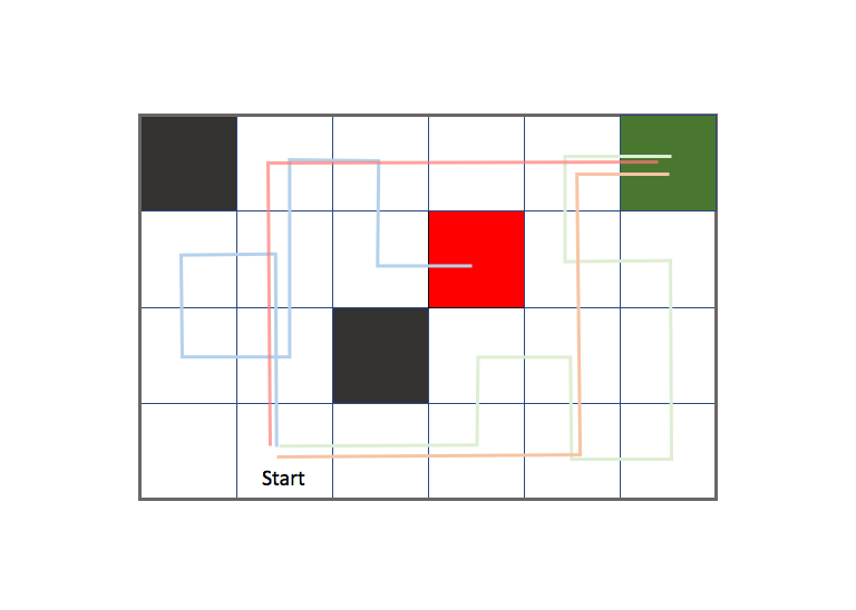
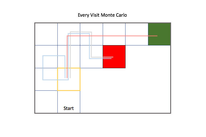
For Monte Carlo learning, we use a collection of complete episodes to approximate the value function. An episode is defined as the agent journey from the initial state to the terminal state, so this approach only works when your environment has a concrete ending. Let's revisit the gridworld example with a more complex environment. As a reminder, the agent can take an action to move up, down, left, or right and the green and red states are terminal states. However, we no longer know the reward for any of the states until we've visited them nor do we know how the transfer function determines the agent's next state (as we did when discussing the Markov Decision Process).
Each colored path is an episode which represents the path an agent took to reach a terminal state.
Previously, we defined $Q\left( {s,a} \right)$ as the expectation of the accumulated reward starting from a given state and performing a given action.
$$ Q\left( {s,a} \right) = E\left[ {R\left( {{S_ t}} \right) + \gamma R\left( {{S_ {t + 1}}} \right) + {\gamma ^2}R\left( {{S_ {t + 2}}} \right) + ...|{S_ t} = s,{A_ t} = a} \right] $$
For Monte Carlo approximation, we'll replace this expectation with the mean value of accumulated rewards over all episodes. These accumulated rewards are sometimes referred to collectively as a return, defined as ${G_t}$ below.
$$ {G_t} = {R_t} + \gamma {R_{t + 1}} + ... + {\gamma ^{T - 1}}{R_T} $$
For example, suppose we wanted to calculate the value of starting in the state highlighted in yellow, and then taking an action to move right. There were two episodes in which we visited this state and proceeded by moving right.
Actually, it's important to note that we don't know what action the agent took during each episode unless I explicitly provided that information, since the environment exhibits stochastic behavior and our transfer function doesn't always bring the agent to the intended state. For simplicity's sake, in this example I will also suppose that our agent took the action to move right for both episodes.
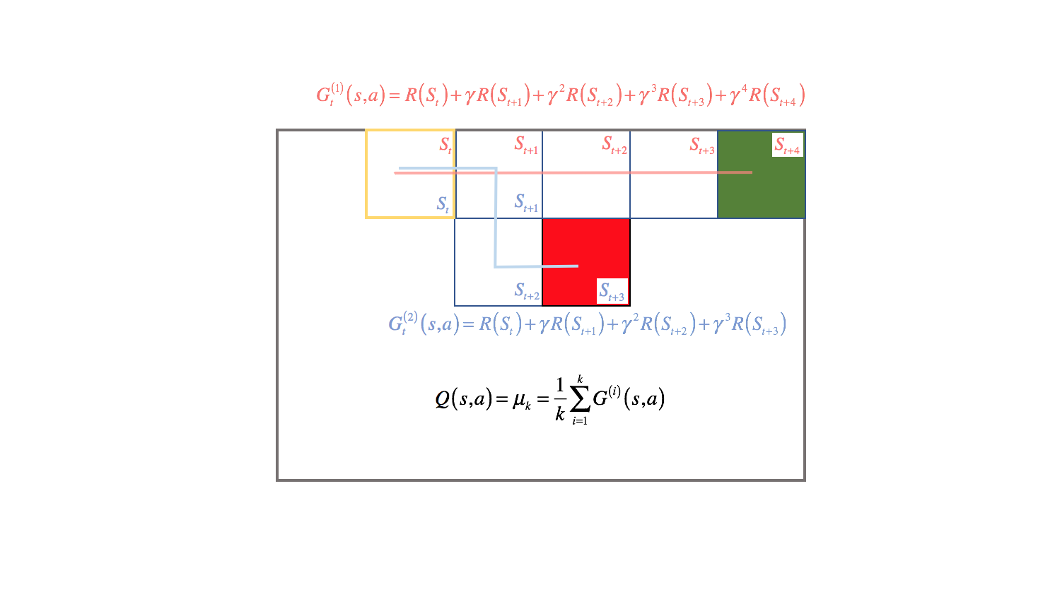
We can calculate the value of existing in the highlighted state and moving right for both episodes by the discounted accumulation of reward until the agent reaches a terminal state. Then, we can approximate a general value for moving right from the highlighted state by taking the mean of all episodic returns.
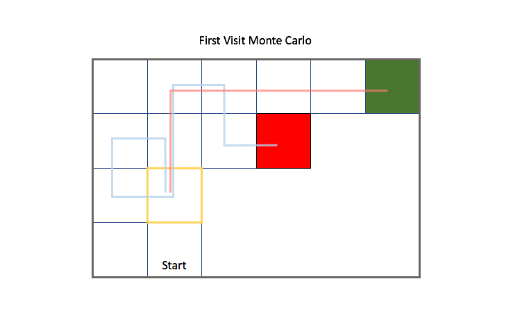
When evaluating all of the states within an environment, there's two general ways to approach this. One approach is to consider the future trajectory of a state from the point of first visit of the state for each episode; this is known as First Visit Monte Carlo Evaluation. We only consider trajectories from a state for the first visit by the agent.
The second approach is to consider the future trajectories of a state for all times that the state is visited for each episode; this is known as Every Visit Monte Carlo Evaluation. Notice how in this case we also consider the gray trajectory starting from the highlighted state after the blue trajectory passes back through the state.
Earlier, we established our approximation for the action-value function as the mean return for each state-action pair over all episodes. In order to learn after each episode, we can rewrite our calculation for the mean in an incremental fashion.
$$ Q\left( {s,a} \right) = {\mu_ k} = \frac{1}{k}\sum\limits_ {i = 1}^k {{G^{\left( i \right)}}\left( {s,a} \right)} $$
First, we'll pull our latest episode outside of the summation.
$$ {\mu_k} = \frac{1}{k}\left( {{G^{\left( k \right)}}\left( {s,a} \right) + \sum\limits_{i = 1}^{k - 1} {{G^{\left( i \right)}}\left( {s,a} \right)} } \right) $$
We can then express the summation as a repeated mean.
$$ {\mu_k} = \frac{1}{k}\left( {{G^{\left( k \right)}}\left( {s,a} \right) + \left( {k - 1} \right){\mu_{k - 1}}} \right) $$
With a little more rearrangement, we arrive at a definition for the mean which we can update incrementally using the current episodic state-action values combined with the total approximated state-action values.
$$ {\mu_k} = {\mu_{k - 1}} + \frac{1}{k}\left( {{G^{\left( k \right)}}\left( {s,a} \right) - {\mu_{k - 1}}} \right) $$
Each time we visit a state in an episode, we can total the reward accumulated from that state onward and upon reaching a terminal state, we can update our value function approximation. We can also incrementally calculate a running mean (forgetting older values over time) by substituting $\frac{1}{k}$ for a constant value, $\alpha$, in cases where the environment state change over time. This results in more recent experiences holding more weight when approximating the true action value function.
$$ {\mu_k} = {\mu_{k - 1}} + \alpha \left( {{G^{\left( k \right)}}\left( {s,a} \right) - {\mu_{k - 1}}} \right) $$
Recall that ${\mu_k}$ is our estimate for the true value function, ${{Q}\left( {s,a} \right)}$, given what we've learned from $k$ episodes. In general terms, this update equation allows us to compare our previous estimate, ${\mu_ {k - 1}}$, to the return from the latest episode, $G^{\left( k \right)}$, and update our guess accordingly.
$$ Q\left( {s,a} \right) \leftarrow Q\left( {s,a} \right) + \alpha \left( {{G^{\left( k \right)}}\left( {s,a} \right) - Q\left( {s,a} \right)} \right) $$
Temporal difference approach
Initially, our estimated value function is arbitrarily defined - often we assume that every state-action pair has zero value, although you can also initialize the value function to a small positive number in order to encourage exploration (known as "optimism in the face of uncertainty"). However, as our agent explores an environment and accumulates experiences, we can use these experiences to update our guess of the true value function. The value function represents the reward of completing an action, and accumulating future rewards by following a set policy. Thus, our estimated value function signals how much reward we expect to accumulate from entering a state and performing some action. In the Monte Carlo approach previously discussed, we simulated complete episodes and would then back-calculate the value of each state-action pair executed during the episode. Since we ran the simulation to completion (ie. our agent reached a terminal state), we could easily calculate the future accumulated reward from any point during the simulation.
However, the Monte Carlo approach requires us to run complete episodes before we can update our estimated value function. In Monte Carlo learning, we would update the value of a state-action pair by comparing the historical mean to the episodic return, and take a step in the direction which would minimize this difference.
Temporal difference learning provides an online learning approach, allowing us to update the estimated value function during a single episode. As the name implies, we update our value function by looking at the difference of the estimated value of a state-action pair at two different points in time (temporal difference). More concretely, we'll compare a current estimate for the value of a state-action pair to a more informed future estimate after the agent has gained more experience within the environment.
For example, upon arriving at some state we'll look at the reward the agent immediately collects plus the expected future returns upon entering a subsequent state, $s'$, via performing some action, and compare this with our previous estimate for the value of this state-action pair.
$$ Q\left( {s,a} \right) \leftarrow Q\left( {s,a} \right) + \alpha \left( {\left( {{R_t} + \gamma Q\left( {s',a'} \right)} \right) - Q\left( {s,a} \right)} \right) $$
The expression ${R_t} + \gamma Q\left( {s',a'}\right)$ is known as the TD target, and represents a better approximation for $Q\left( {s,a} \right)$ given the fact that it replaces an estimated reward received from existing in state $s$ with the actual reward. In this instance, the TD target is one step ahead of the state-action pair value that we're updating, but this can be extended to look $n$ steps ahead when approximating $Q\left( {s,a} \right)$. Comparing the TD target to the previous approximation for $Q\left( {s,a} \right)$ yields what is known as the TD error, $\delta_t $; our update function takes a step in the direction which minimizes the TD error.
$$ \delta_t = {\left( {{R_t} + \gamma Q\left( {s',a'} \right)} \right) - Q\left( {s,a} \right)} $$
This approach to learning allows us to make updates before we have knowledge of the final outcome, which is clearly advantageous when learning in a non-terminating environment.
A hybrid approach
To extend our TD expression to look $n$ steps ahead, we simply need to update our TD target. Remember, the TD target represents a more informed approximation for the value of a state-action pair by incorporating observed future returns. For $n=1$, we take one step forward, observe the reward and combine it with our estimate of future returns from that point onward, and assign this as the TD target for the original state. For $n=2$, we follow the same procedure expect this time we take two steps forward, observing the reward collected at each state.
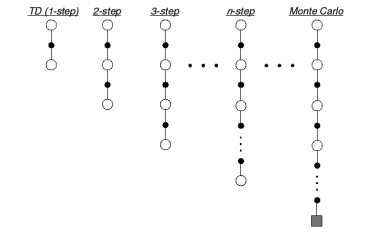
Photo by Richard Sutton
In this diagram, white circles represent states, black circles represent reward collected, and the square represents a terminal state.
Generally, the TD target for $TD\left( n \right)$ is as follows:
$$ {R_t} + \gamma {R_{t + 1}} + ... + {\gamma ^{n - 1}}{R_{t + n - 1}} + {\gamma ^n}Q\left( {s',a'} \right) $$
If we were to look all the way forward to $n = \infty$, we would arrive at the Monte Carlo approach for learning, where we simply look at the discounted sum of rewards after leaving some state $s$ via action $a$.
As we increase $n$, we're including more observations from the actual environment which reduces the bias in our estimate (see following section on comparing learning methods). However, because each next state is a result of a stochastic process, the variance increases. For different environments, there exist different values of $n$ which can most efficiently propagate information backwards. A more robust approach would be to use a TD target which efficiently considers all $n$ at once.
This more robust approach is referred to as the $TD\left( \lambda \right)$ approach which combines all $n$-step returns as a geometric weighted sum, decayed by a factor of $\lambda$, as shown in the diagram below. We specifically choose to use a geometric sum for the sake of computational efficiency.
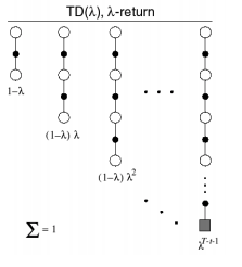
Photo by Richard Sutton
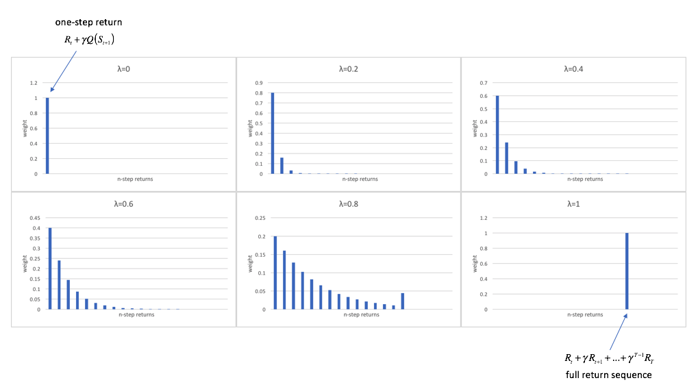
Setting $\lambda = 0$, only the one-step return has a non-zero weight and thus this is equivalent to the $TD\left( 0 \right)$ method. Setting $\lambda = 1$, only the full return sequence has a non-zero weight and thus this is equivalent to the Monte Carlo method. The figure below shows weighting for each of the $n$-step returns from $n=1$ (the one-step return) through $n=\infty$ (the full return sequence), according to various values of $\lambda$.
The $TD\left( \lambda \right)$ target, $G_t^\lambda$, which aggregates $n$-step returns for all values of $n$, may be written as
$$G_t^\lambda = \left( {1 - \lambda } \right)\sum\limits_{n = 1}^\infty {{\lambda ^{n - 1}}} G_t^{\left( n \right)} $$
where $G_t^{\left( n \right)}$ represents the $n$-step return. The result is a more robust value approximation model. Tuning the parameter $\lambda$ generalizes to more cases much better than you would observe tuning $n$.
Up until now, I've been discussing temporal difference learning from the perspective of a forward-view, where we assign the value of a state-action pair by observing what happens in the following steps.
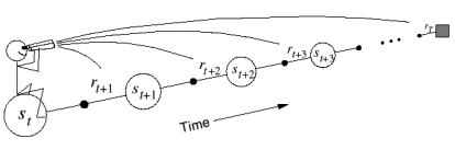
Photo by Richard Sutton
However, in order to implement this forward-view approach, we'd need to wait until the end of each episode before we perform our updates. Fortunately, we can reframe this perspective to look at a backward-view that would allow us to update previously visited states upon sufficient exploration. For example, in the case of $TD\left(n\right)$ learning, each step we take along a trajectory allows us to update the value of the state $n$ steps prior to our current state.
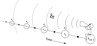
Photo by Richard Sutton
In doing this, we can send back the longer-term result of actions in previous states. However, this introduces the credit assignment problem. When considering updates for multiple $n$-steps back, how do we know which previous actions had an influence on the reward accumulated at the current timestep?
A frequency heuristic would assign credit to the states which we had previously visited most frequently. This would be assuming that the states we visited most often are the most likely influence on our current outcome. A recency heuristic would assign credit to the states which we had visited most recently. This would be assuming that our current outcomes are most likely influenced by the states we visited most recently. An eligibility trace combines both of these heuristics by increasing the credit assigned to a state by a fixed amount every time the state is visited, and slowly decaying that credit over time as shown in the photo below.
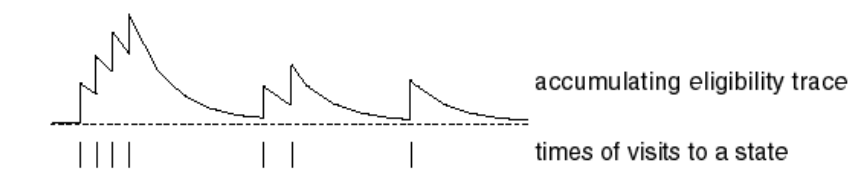
Photo by Richard Sutton
As our agent explores the environment, we update our state-action value function in the direction which minimizes TD error, scaled by the eligibility trace for each state updated. This allows us to focus our updates on the states which we believe resulted in future returns.
We'll initialize the eligibility for all state-action pairs to be zero at time $t=0$.
$$ {E_0}\left( {s,a} \right) = 0 $$
At each time step, all state-action pair eligibility traces are decayed by a factor of $\gamma$. Further, we increment the eligibility of a state-action pair by one each time the pair is visited.
$$ {E_t}\left( {s,a} \right) = \gamma \lambda {E_{t - 1}}\left( {s,a} \right) + {\bf{1}}\left( {{S_t} = s,{A_t} = a} \right) $$
This allows us to perform updates to state-action pairs, at each timestep, in proportion to their eligibility, ${E_t}\left( {s,a} \right)$, and the TD error, $\delta _t$.
$$ {\delta_ t} = {R_ {t + 1}} + \gamma Q\left( {{S_ {t + 1}},{A_ {t + 1}}} \right) - Q\left( {{S_ t},{A_ t}} \right) $$
$$ Q\left( {s,a} \right) \leftarrow Q\left( {s,a} \right) + \alpha {\delta _ t}{E_ t}\left( {s,a} \right) $$
While our TD error compares only a one-step lookahead to our current estimate, we have the capability to send back error to any state-action pair with a non-zero eligibility.
Comparing learning methods
Bias versus variance trade-off
When performing Monte Carlo learning, we updated our estimated value function based solely on experience from previous episodes; the value of a given state-action pair is calculated as the mean return over all episodes. Thus, we introduce zero bias with this approach. However, the returns from any given episode are an accumulation of stochastic transitions, which can introduce a high level of variance into our estimated value function.
On the contrary, when updating our estimated value function using temporal difference learning we use one step of experience combined with an estimate of the future returns from that point onward (collectively known as the TD target). In this case, our estimation of future returns introduces bias; however, this approach has much less variance since we only have one stochastic transition.
Markov environments
In both learning methods (TD and Monte Carlo), we update our estimate of the value function by comparing our estimate to some target, and we adjust our estimate to be closer to the target.
In TD learning, our target is defined as
$$ {R_t} + \gamma Q\left( {s',a'} \right) $$
for the case of $TD\left( 0 \right)$.
In Monte Carlo learning, our target is defined as the episodic return
$$ {R_t} + \gamma {R_{t + 1}} + ... + {\gamma ^\infty }{R_\infty } $$
where we simply discount all of the returns subsequent to a state until the terminal state is reached.
The Markov property mandates that the conditional probability of future states depend only on the current state, not on the sequence of states which preceded it. Earlier, when looking at the value of sequences of states, we used this property to collapse the entire future value of a trajectory into a value assigned to a single state. The value of any given state implicitly accounted for the future reward accumulated when following some policy. In the temporal difference approach for learning, we similarly assigned our TD target as an estimated value that considers the future sequence of states. Because TD learning exploits this Markov property, it is generally more efficient than Monte Carlo learning in Markov environments.
Epsilon-greedy exploration
As our agent explores the environment and builds an understanding for the value of its actions, we gain the ability to make "smarter" decisions. However, if we prematurely optimize our policy before fully exploring the environment, we may converge to a sub-optimal policy.
Suppose you're presented two doors, which you can open and keep whatever reward lies on the other side. You open Door A and find nothing. Next, you open Door B and get $5. Given what you've learned so far, the "optimal" policy would instruct you to continue opening Door B and forget that Door A exists entirely. However, if this occurs in a stochastic environment, how can we be so sure that there's no value in opening Door A after only one try?
The simplest way to address this problem is known as epsilon-greedy exploration. The greedy action represents that which our policy would recommend for optimal results, and we'll follow this policy with a probability of $1 - \epsilon$. However, we'll resort to random choice with a probability of $\epsilon$, allowing us to sometimes make "stupid" choices for the sake of exploration. Often, these random explorations will discover a more valuable state than our policy had knowledge of, and we can adjust our policy accordingly.
However, while this $\epsilon$-greedy policy is very valuable for encouraging the agent to explore an environment, ultimately we'd like to converge on a greedy policy that always makes the optimal decision (ie. without random exploration). This trade-off is known generally as exploration versus exploitation, which refers to the balance between encouraging your agent to explore the environment and encouraging your agent to make smart decisions within the environment.
One idea to address this tradeoff is Greedy in the Limit with Infinite Exploration (GLIE). GLIE mandates that 1) all state-action pairs are explored infinitely many times and 2) the policy eventually converges on a greedy policy. We could apply the principles of GLIE to an $\epsilon$-greedy policy by simply decaying $\epsilon$ over time.
Summary
In this post, we introduced $Q\left( {s,a} \right)$ as a way for determining the optimal policy without knowledge of the underlying system dynamics. This allows us to learn from the environment, rather than just plan.
We then discussed two main approaches for updating $Q\left( {s,a} \right)$ as our agent explores an environment:
Monte Carlo
- Learn from complete episodes.
- High variance, zero bias.
- Full lookahead.
Temporal Difference
- Learn from incomplete/ongoing episodes.
- High bias, low variance.
- Short-term lookahead combined with a guess.
Lastly, we introduced a technique which presents a hybrid of the two methods, which leads to more efficient learning. In my next post, I'll discuss specific implementations of these general methods.
Further reading
- RL Course by David Silver - Lecture 4: Model-Free Prediction
- RL Course by David Silver - Lecture 5: Model Free Control
- Reinforcement Learning: An Introduction by Richard S. Sutton and Andrew G. Barto
Note: In his lectures, David Silver assigns reward as the agent leaves a given state. In my blog posts, I assign reward as the agent enters a state, as it is what makes most sense to me. In one of his lectures he makes this distinction and states that either way is valid, it's just a matter of notation. Thus, if you're following along with David Silver's notes, you might find small deviations between his equations and the ones on this blog. If you're confused, feel free to ask questions in the comments section.