Implementations of Monte Carlo and Temporal Difference learning.

In the previous post, I discussed two different learning methods for reinforcement learning, Monte Carlo learning and temporal difference learning. I then provided a unifying view by considering $n$-step TD learning and establishing hybrid learning method, $TD\left( \lambda \right)$. These methods are mainly focused on how to approximate a value function from experience. I introduced a new value function, $Q\left( {s,a} \right)$, that looks at the value of state-action pairs in order to achieve model-free learning. For all approaches, learning takes place by policy iteration, as shown below.
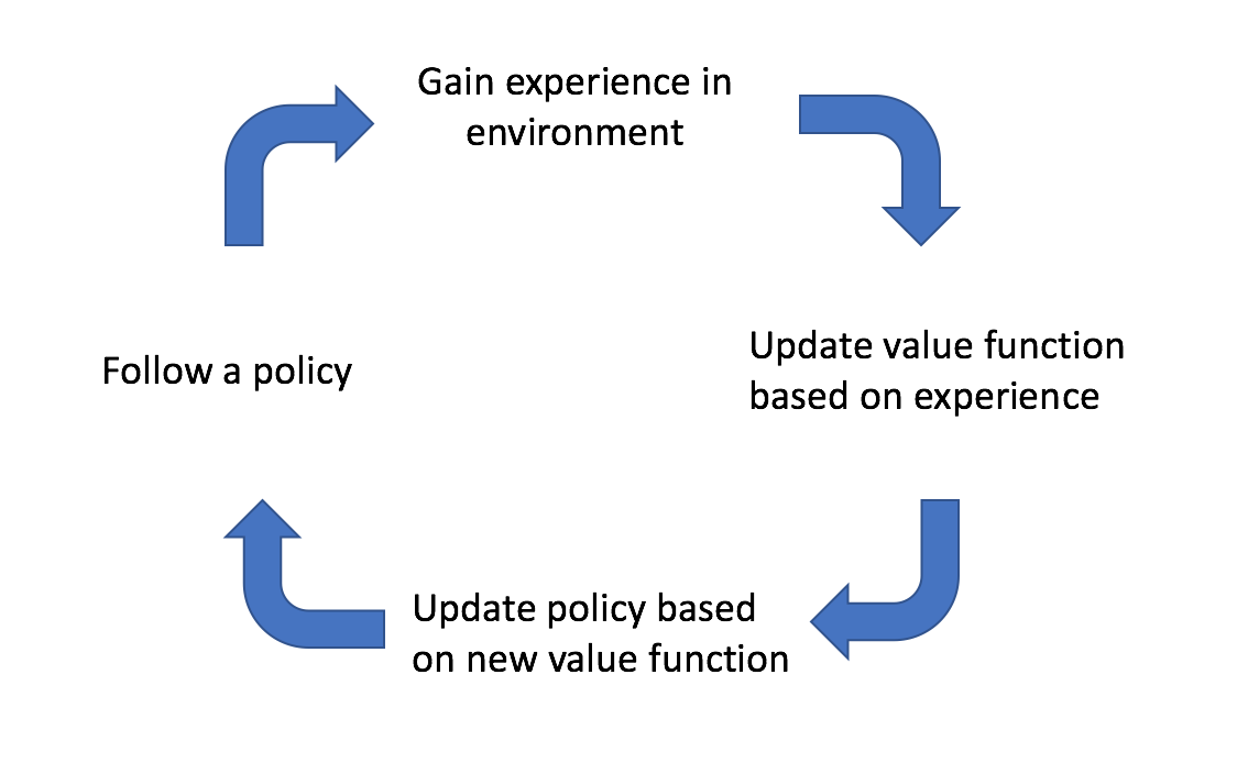
We start off by following an initial policy and explore the environment. As we observe the results of our actions, we can update our estimate of the true value function that describes the environment. We can then update our policy by querying the best actions to take according to our newly estimated value function. Ideally, this cycle continues until we've sufficiently explored the environment and have converged on an optimal policy.
In this post, I'll discuss specific implementations of the Monte Carlo and TD approach to learning. However, I first must introduce the concept of on-policy and off-policy learning. A method is considered on-policy if the agent follows the same policy which it is iteratively improving. However, there are cases where it would be more useful to have the agent follow a behavior policy while learning a target policy. Such methods, where the agent doesn't follow the same policy that it is learning, are considered off-policy.
Monte Carlo learning
The Monte Carlo approach approximates the value of a state-action pair by calculating the mean return from a collection of episodes.
GLIE Monte-Carlo
GLIE Monte-Carlo is an on-policy learning method that learns from complete episodes. For each state-action pair, we keep track of how many times the pair has been visited with a simple counter function.
$$ N\left( {{S_t},{A_t}} \right) \leftarrow N\left( {{S_t},{A_t}} \right) + 1 $$
For each episode, we can update our estimated value function using an incremental mean.
$$ Q\left( {{S_t},{A_t}} \right) \leftarrow Q\left( {{S_t},{A_t}} \right) + \frac{1}{{N\left( {{S_t},{A_t}} \right)}}\left( {{G_t} - Q\left( {{S_t},{A_t}} \right)} \right) $$
Here, $G_t$ either represents the return from time $t$ when the agent first visited the state-action pair, or the sum of returns from each time $t$ that the agent visited the state-action pair, depending on whether you are using first-visit or every-visit Monte Carlo.
We'll adopt an $\epsilon$-greedy policy with $\epsilon=\frac{1}{k}$ where $k$ represents the number of episodes our agent has learned from.
Temporal difference learning
The temporal difference approach approximates the value of a state-action pair by comparing estimates at two points in time (thus the name, temporal difference). The intuition behind this method is that we can formulate a better estimate for the value of a state-action pair after having observed some of the reward that our agent accumulates after having visited a state and performing a given action.
Sarsa
Sarsa is an on-policy $TD\left(0 \right)$ learning method. The name refers to the State-Action-Reward-State-Action sequence that we use to update our action value function, $Q\left( {s,a} \right).$
We start off in state $S$ and perform action $A$. This state-action pair yields some reward $R$ and brings us to a new state, $S'$. We then follow our policy to perform action $A'$ and look up the value of this future trajectory according to $Q\left( {S',A'} \right)$ (taking advantage of the fact that we define the value of a state-action pair to incorporate the value of the entire future sequence of states following our policy).
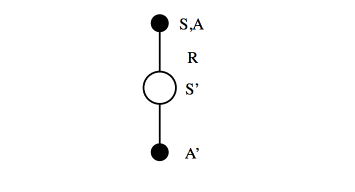
Photo by Richard Sutton
We'll define our policy as $\epsilon$-greedy with respect to $Q\left( {s,a} \right)$, which means that our agent will have a $1 - \epsilon$ probability of performing the optimal action in state $S'$ and an $\epsilon$ probability of performing a random exploratory action.
The value function update equation may be written as
$$ Q\left( {S,A} \right) \leftarrow Q\left( {S,A} \right) + \alpha \left( {\left( {R + \gamma Q\left( {S',A'} \right)} \right) - Q\left( {S,A} \right)} \right) $$
where we include one step of experience combined with a discounted estimate for future returns as our TD target.
Q-learning
Q-learning is an off-policy $TD\left(0 \right)$ learning method where the agent's next action is chosen according to a behavior policy but we evaluate state-action pairs according to a target policy. This has the effect of allowing our agent to explore while maintaining the highest possible accuracy when comparing our expected state-action value to a target.
We'll define our behavior policy, the policy that determines the agent's actions, as $\epsilon$-greedy with respect to $Q\left( {s,a} \right)$. However, we'll also define a target policy as greedy with respect to $Q\left( {s,a} \right)$.
Rather than looking at a sequence of State-Action-Reward-State-Action, we instead take a sequence of State-Action-Reward-State and refer to our target policy for the subsequent action. Because our target policy is greedy, there is no stochastic behavior ($\epsilon$ exploration) present to degrade the accuracy of our TD target.
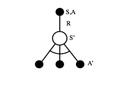
Photo by Richard Sutton
The value function update equation for Q-learning may be written as
$$ Q\left( {S,A} \right) \leftarrow Q\left( {S,A} \right) + \alpha \left( {\left( {R + \gamma \mathop {\max }\limits_{a'} Q\left( {S',A'} \right)} \right) - Q\left( {S,A} \right)} \right) $$
where we similarly include one step of experience combined with a discounted estimate for future returns as our TD target; however, we've removed the exploratory behavior from our estimate for future returns in favor of selecting the optimal trajectory, increasing the accuracy of our TD target.
Hybrid approach to learning
$n$-step Sarsa
So far, we've discussed methods which seek a more informed valuation of a state-action pair by two main approaches, a one-step lookahead combined with a guess (the temporal difference approach) and a full sequence lookahead (the Monte Carlo approach). Let us now consider the spectrum of algorithms that lie between these two methods by expanding our Sarsa implementation to include $n$-step returns.
The general Sarsa algorithm considers the case of $n=1$, where our more informed valuation of a state-action pair $q_t^{\left( 1 \right)}$ at time $t$ may be written as:
$$ q_t^{\left( 1 \right)} = {R_t} + \gamma Q\left( {{S_{t + 1}}} \right) $$
At the other end of the spectrum, the Monte Carlo approach, which considers a full sequence of observed rewards until the agent reaches a terminal timestep $T$, may be written as:
$$ q_t^{\left( \infty \right)} = {R_t} + \gamma {R_{t + 1}} + ... + {\gamma ^{T - 1}}{R_T} $$
However, we could develop $q_t^{\left( n \right)}$ to generally represent a target value which incorporates $n$ steps of experience combined with a guess for the value of the future trajectory from that point onward.
$$ q_t^{\left( n \right)} = {R_t} + \gamma {R_{t + 1}} + {\gamma ^{n - 1}}{R_{t + n - 1}} + {\gamma ^n}Q\left( {{S_{t + n}}} \right) $$
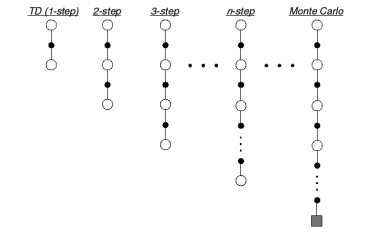
Photo by Richard Sutton
The $n$-step Sarsa implementation is an on-policy method that exists somewhere on the spectrum between a temporal difference and Monte Carlo approach.
The value function update equation may be written as
$$ Q\left( {S,A} \right) \leftarrow Q\left( {S,A} \right) + \alpha \left( {q_t^{\left( n \right)} - Q\left( {S,A} \right)} \right) $$
where $q_t^{\left( n \right)}$ is the general $n$-step target we defined above.
Sarsa$\left(\lambda\right)$
In the last post, I discussed a general method for combining the information from all of the $n$-step returns into a single collective return by calculating the geometric sum of the returns. Recall that this approach is more robust than simply choosing the optimal $n$-step return, given the fact that the optimal $n$-step return varies according to the situation.
Using a weight of $\left( {1 - \lambda } \right){\lambda ^{n - 1}}$, we can efficiently combine all $n$-step returns into a target value, $q_t^\lambda$.
$$ q_t^\lambda = \left( {1 - \lambda } \right)\sum\limits_{n = 1}^\infty {{\lambda ^{n - 1}}} q_t^{\left( n \right)} $$
The forward-view Sarsa$\left(\lambda\right)$ simply adjusts our estimated value function towards the $q_t^\lambda$ target.
$$ Q\left( {{S_t},{A_t}} \right) \leftarrow Q\left( {{S_t},{A_t}} \right) + \alpha \left( {q_t^\lambda - Q\left( {{S_t},{A_t}} \right)} \right) $$
This method will, for each state-action pair, combine the returns from a one-step lookahead, two-step lookahead, ..., $n$-step lookahead, all the way to a full reward sequence lookahead, aggregate the returns by a geometric sum, and adjust the original estimate towards this new aggregated lookahead.
However, we need to develop a backward-view algorithm in order to enable our agent to learn online during each episode. Otherwise, we'd need to wait until the agent reaches a terminal state to do the forward-view algorithm described above. To do this, we'll need to replace our $n$-step aggregation approach with eligibility traces, a way of keeping track of which previously visited states are likely to be responsible for the reward accumulated (covered in more detail in the previous post).
As covered in the last post, we'll initialize all eligibilities to zero, increment the eligibility of visited states, and decay all eligibilities at each time step.
$$ {E_0}\left( {s,a} \right) = 0 $$
$$ {E_t}\left( {s,a} \right) = \gamma \lambda {E_{t - 1}}\left( {s,a} \right) + {\bf{1}}\left( {{S_t} = s,{A_t} = a} \right) $$
Our value function is updated in proportion to both the TD error and the eligilibilty trace.
$$ Q\left( {s,a} \right) \leftarrow Q\left( {s,a} \right) + \alpha {\delta _ t}{E_ t}\left( {s,a} \right) $$
This method is an on-policy approach, meaning that next actions are selected according to the learned policy.