An overview of semantic image segmentation.

In this post, I'll discuss how to use convolutional neural networks for the task of semantic image segmentation. Image segmentation is a computer vision task in which we label specific regions of an image according to what's being shown.

"What's in this image, and where in the image is it located?"

Jump to:

• Representing the task
• Constructing an architecture
  • Methods for upsampling
  • Fully convolutional networks
  • Adding skip connections
  • Advanced U-Net variants
  • Dilated convolutions
• Defining a loss function
• Common datasets and segmentation competitions
• Further reading

More specifically, the goal of semantic image segmentation is to label each pixel of an image with a corresponding class of what is being represented. Because we're predicting for every pixel in the image, this task is commonly referred to as dense prediction.

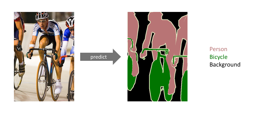
An example of semantic segmentation, where the goal is to predict class labels for each pixel in the image. (Source)

One important thing to note is that we're not separating instances of the same class; we only care about the category of each pixel. In other words, if you have two objects of the same category in your input image, the segmentation map does not inherently distinguish these as separate objects. There exists a different class of models, known as instance segmentation models, which do distinguish between separate objects of the same class.

Segmentation models are useful for a variety of tasks, including:

• Autonomous vehicles
  We need to equip cars with the necessary perception to understand their environment so that self-driving cars can safely integrate into our existing roads.

A real-time segmented road scene for autonomous driving. (Source)

• Medical image diagnostics
  Machines can augment analysis performed by radiologists, greatly reducing the time required to run diagnositic tests.

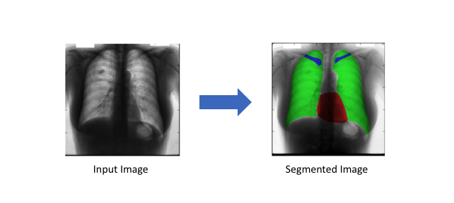
A chest x-ray with the heart (red), lungs (green), and clavicles (blue) are segmented. (Source)

Representing the task

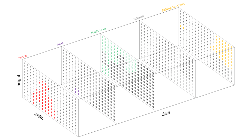
Simply, our goal is to take either a RGB color image ($height\times width\times 3$) or a grayscale image ($height\times width\times 1$) and output a segmentation map where each pixel contains a class label represented as an integer ($height\times width\times 1$).

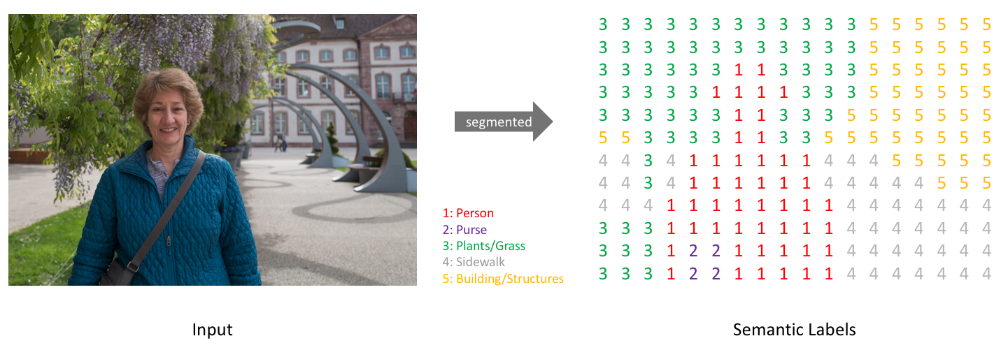
Note: For visual clarity, I've labeled a low-resolution prediction map. In reality, the segmentation label resolution should match the original input's resolution.

Similar to how we treat standard categorical values, we'll create our target by one-hot encoding the class labels - essentially creating an output channel for each of the possible classes.

A prediction can be collapsed into a segmentation map (as shown in the first image) by taking the argmax of each depth-wise pixel vector.

We can easily inspect a target by overlaying it onto the observation.

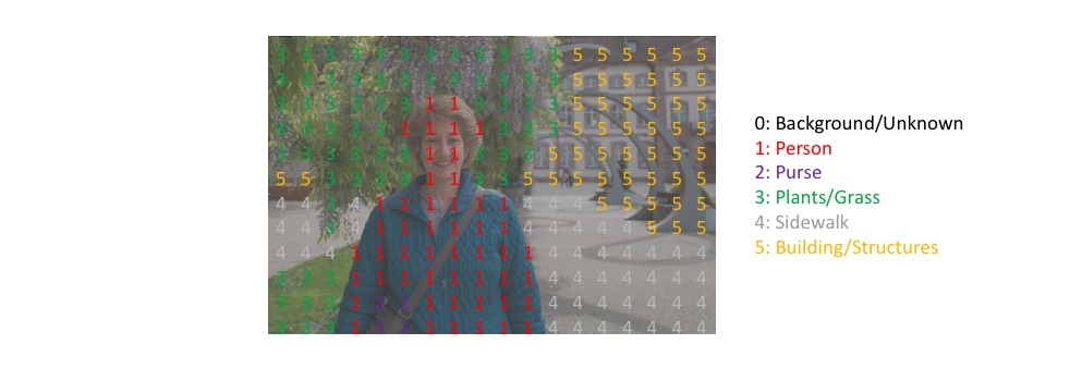
When we overlay a single channel of our target (or prediction), we refer to this as a mask which illuminates the regions of an image where a specific class is present.

Constructing an architecture

A naive approach towards constructing a neural network architecture for this task is to simply stack a number of convolutional layers (with same padding to preserve dimensions) and output a final segmentation map. This directly learns a mapping from the input image to its corresponding segmentation through the successive transformation of feature mappings; however, it's quite computationally expensive to preserve the full resolution throughout the network.

Image credit

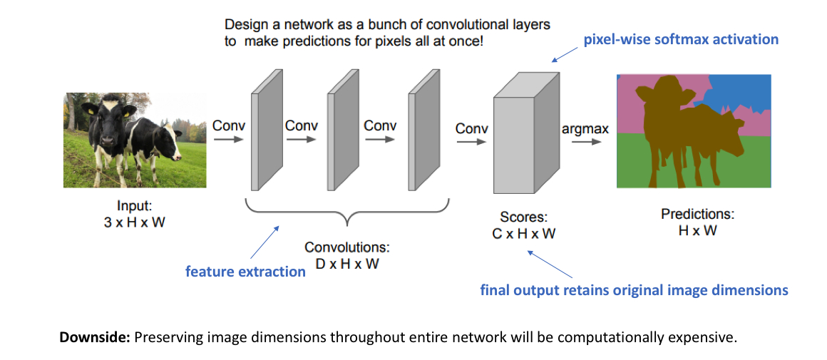
Recall that for deep convolutional networks, earlier layers tend to learn low-level concepts while later layers develop more high-level (and specialized) feature mappings. In order to maintain expressiveness, we typically need to increase the number of feature maps (channels) as we get deeper in the network.

This didn't necessarily pose a problem for the task of image classification, because for that task we only care about what the image contains (and not where it is located). Thus, we could alleviate computational burden by periodically downsampling our feature maps through pooling or strided convolutions (ie. compressing the spatial resolution) without concern. However, for image segmentation, we would like our model to produce a full-resolution semantic prediction.

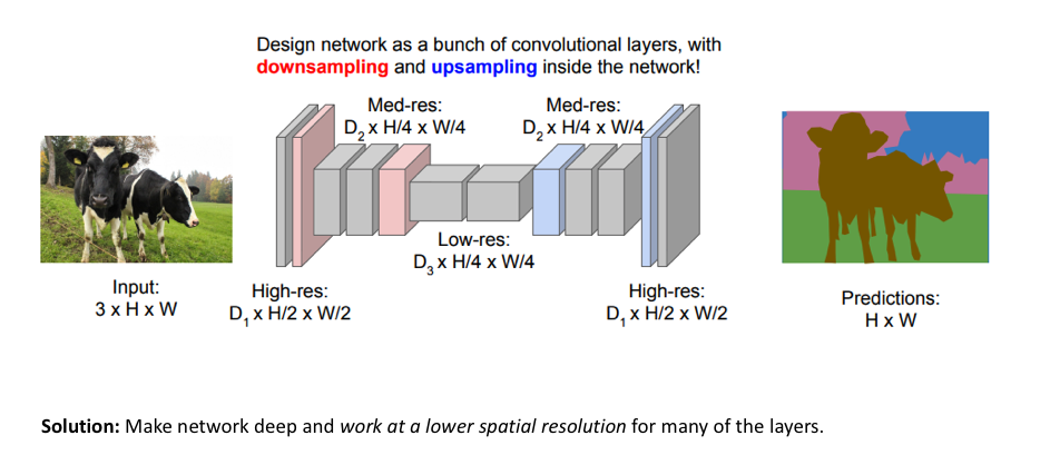
One popular approach for image segmentation models is to follow an encoder/decoder structure where we downsample the spatial resolution of the input, developing lower-resolution feature mappings which are learned to be highly efficient at discriminating between classes, and the upsample the feature representations into a full-resolution segmentation map.

Image credit

Methods for upsampling

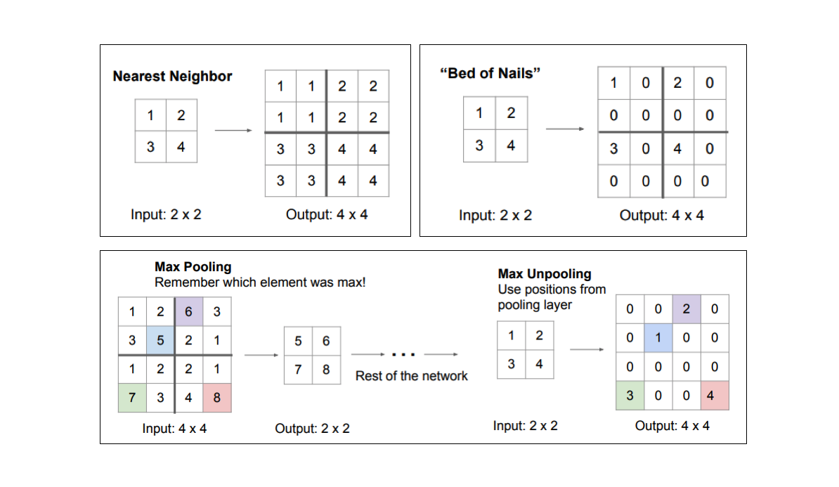
There are a few different approaches that we can use to upsample the resolution of a feature map. Whereas pooling operations downsample the resolution by summarizing a local area with a single value (ie. average or max pooling), "unpooling" operations upsample the resolution by distributing a single value into a higher resolution.

Image credit

However, transpose convolutions are by far the most popular approach as they allow for us to develop a learned upsampling.

Image credit

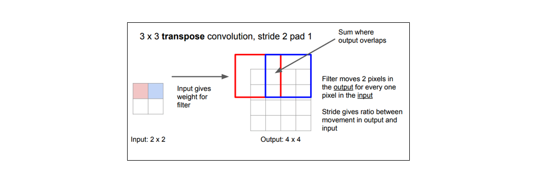
Whereas a typical convolution operation will take the dot product of the values currently in the filter's view and produce a single value for the corresponding output position, a transpose convolution essentially does the opposite. For a transpose convolution, we take a single value from the low-resolution feature map and multiply all of the weights in our filter by this value, projecting those weighted values into the output feature map.

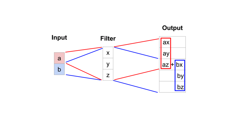
A simplified 1D example of upsampling through a transpose operation. (Source)

For filter sizes which produce an overlap in the output feature map (eg. 3x3 filter with stride 2 - as shown in the below example), the overlapping values are simply added together. Unfortunately, this tends to produce a checkerboard artifact in the output and is undesirable, so it's best to ensure that your filter size does not produce an overlap.

Input in blue, output in green. (Source)

Fully convolutional networks

The approach of using a "fully convolutional" network trained end-to-end, pixels-to-pixels for the task of image segmentation was introduced by Long et al. in late 2014. The paper's authors propose adapting existing, well-studied image classification networks (eg. AlexNet) to serve as the encoder module of the network, appending a decoder module with transpose convolutional layers to upsample the coarse feature maps into a full-resolution segmentation map.

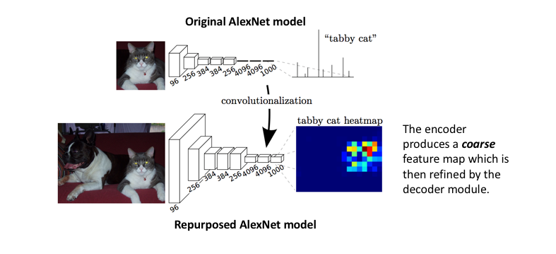
Image credit (with modification)

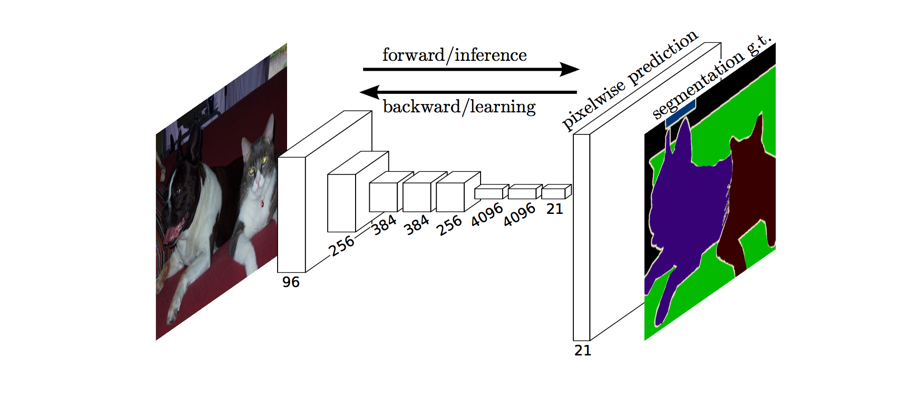
The full network, as shown below, is trained according to a pixel-wise cross entropy loss.

Image credit

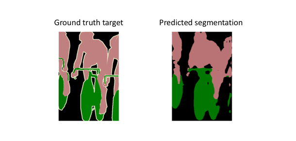
However, because the encoder module reduces the resolution of the input by a factor of 32, the decoder module struggles to produce fine-grained segmentations (as shown below).

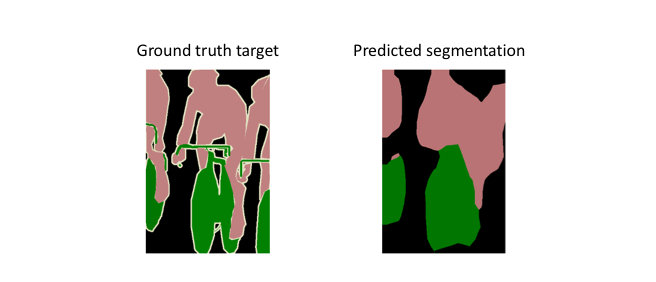
The paper's authors comment eloquently on this struggle:

Semantic segmentation faces an inherent tension between semantics and location: global information resolves what while local information resolves where... Combining fine layers and coarse layers lets the model make local predictions that respect global structure. ― Long et al.

Adding skip connections

The authors address this tension by slowly upsampling (in stages) the encoded representation, adding "skip connections" from earlier layers, and summing these two feature maps.

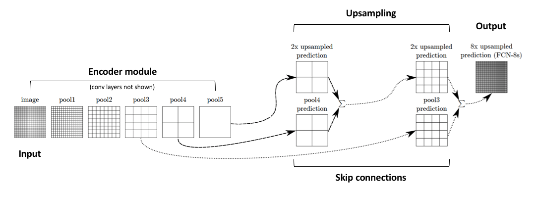
Image credit (with modification)

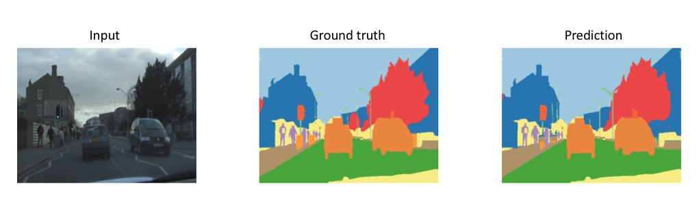
These skip connections from earlier layers in the network (prior to a downsampling operation) should provide the necessary detail in order to reconstruct accurate shapes for segmentation boundaries. Indeed, we can recover more fine-grain detail with the addition of these skip connections.

Ronneberger et al. improve upon the "fully convolutional" architecture primarily through expanding the capacity of the decoder module of the network. More concretely, they propose the U-Net architecture which "consists of a contracting path to capture context and a symmetric expanding path that enables precise localization." This simpler architecture has grown to be very popular and has been adapted for a variety of segmentation problems.

Image credit

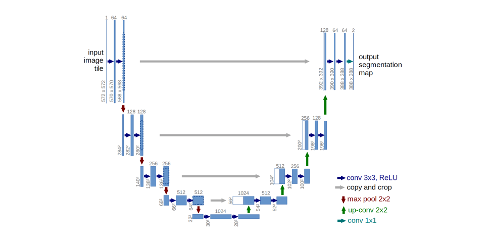
Note: The original architecture introduces a decrease in resolution due to the use of valid padding. However, some practitioners opt to use same padding where the padding values are obtained by image reflection at the border.

Whereas Long et al. (FCN paper) reported that data augmentation ("randomly mirroring and “jittering” the images by translating them up to 32 pixels") did not result in a noticeable improvement in performance, Ronneberger et al. (U-Net paper) credit data augmentations ("random elastic deformations of the training samples") as a key concept for learning. It appears as if the usefulness (and type) of data augmentation depends on the problem domain.

Advanced U-Net variants

The standard U-Net model consists of a series of convolution operations for each "block" in the architecture. As I discussed in my post on common convolutional network architectures, there exist a number of more advanced "blocks" that can be substituted in for stacked convolutional layers.

Drozdzal et al. swap out the basic stacked convolution blocks in favor of residual blocks. This residual block introduces short skip connections (within the block) alongside the existing long skip connections (between the corresponding feature maps of encoder and decoder modules) found in the standard U-Net structure. They report that the short skip connections allow for faster convergence when training and allow for deeper models to be trained.

Expanding on this, Jegou et al. proposed the use of dense blocks, still following a U-Net structure, arguing that the "characteristics of DenseNets make them a very good fit for semantic segmentation as they naturally induce skip connections and multi-scale supervision." These dense blocks are useful as they carry low level features from previous layers directly alongside higher level features from more recent layers, allowing for highly efficient feature reuse.

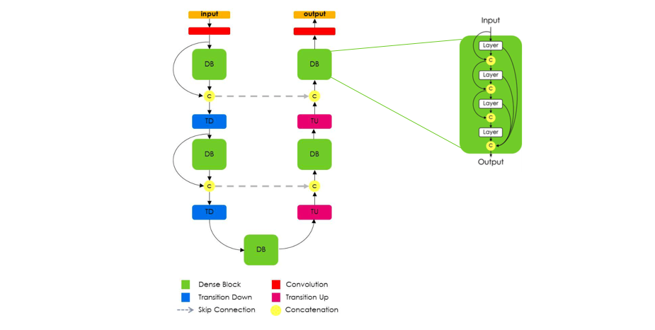
Image credit (with modification)

One very important aspect of this architecture is the fact that the upsampling path does not have a skip connection between the input and output of a dense block. The authors note that because the "upsampling path increases the feature maps spatial resolution, the linear growth in the number of features would be too memory demanding." Thus, only the output of a dense block is passed along in the decoder module.

The FC-DenseNet103 model acheives state of the art results (Oct 2017) on the CamVid dataset.

Dilated/atrous convolutions

One benefit of downsampling a feature map is that it broadens the receptive field (with respect to the input) for the following filter, given a constant filter size. Recall that this approach is more desirable than increasing the filter size due to the parameter inefficiency of large filters (discussed here in Section 3.1). However, this broader context comes at the cost of reduced spatial resolution.

Dilated convolutions provide alternative approach towards gaining a wide field of view while preserving the full spatial dimension. As shown in the figure below, the values used for a dilated convolution are spaced apart according to some specified dilation rate.

Image credit

Some architectures swap out the last few pooling layers for dilated convolutions with successively higher dilation rates to maintain the same field of view while preventing loss of spatial detail. However, it is often still too computationally expensive to completely replace pooling layers with dilated convolutions.

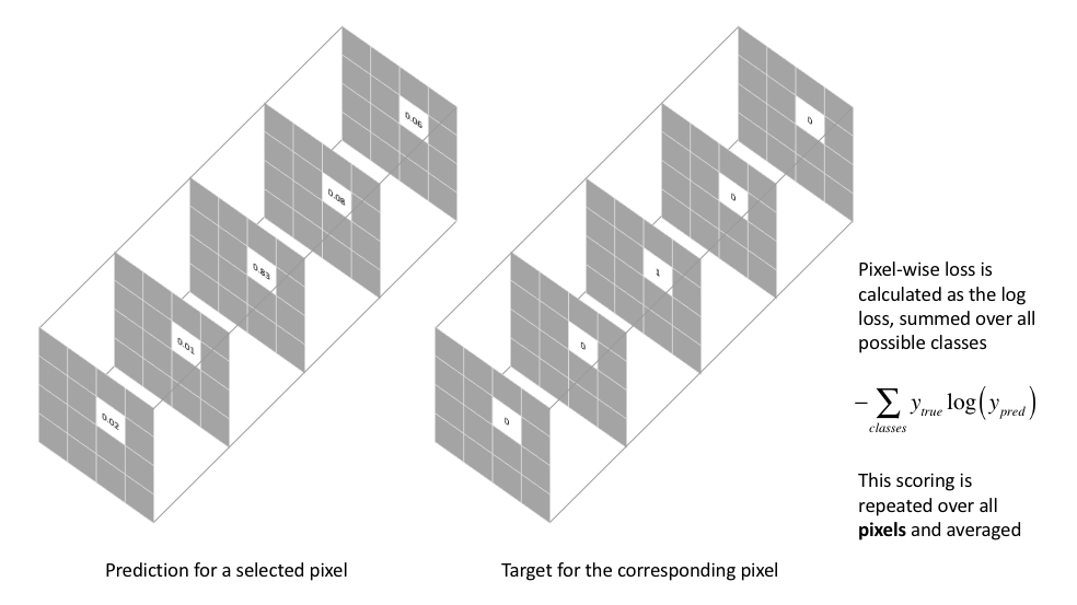
Defining a loss function

The most commonly used loss function for the task of image segmentation is a pixel-wise cross entropy loss. This loss examines each pixel individually, comparing the class predictions (depth-wise pixel vector) to our one-hot encoded target vector.

Because the cross entropy loss evaluates the class predictions for each pixel vector individually and then averages over all pixels, we're essentially asserting equal learning to each pixel in the image. This can be a problem if your various classes have unbalanced representation in the image, as training can be dominated by the most prevalent class. Long et al. (FCN paper) discuss weighting this loss for each output channel in order to counteract a class imbalance present in the dataset.

Meanwhile, Ronneberger et al. (U-Net paper) discuss a loss weighting scheme for each pixel such that there is a higher weight at the border of segmented objects. This loss weighting scheme helped their U-Net model segment cells in biomedical images in a discontinuous fashion such that individual cells may be easily identified within the binary segmentation map.

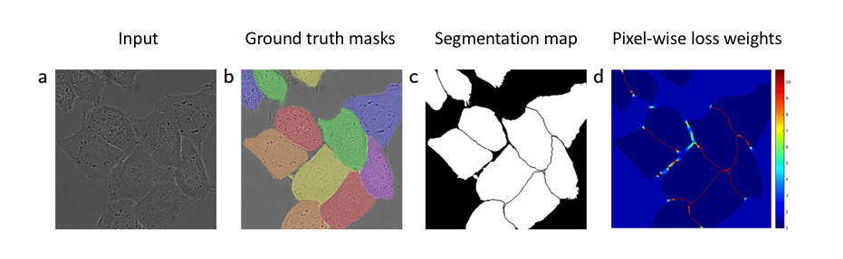
Notice how the binary segmentation map produces clear borders around the cells. (Source)

Another popular loss function for image segmentation tasks is based on the Dice coefficient, which is essentially a measure of overlap between two samples. This measure ranges from 0 to 1 where a Dice coefficient of 1 denotes perfect and complete overlap. The Dice coefficient was originally developed for binary data, and can be calculated as:

$$Dice=\frac{2\left|A\cap B\right|}{\left|A\right|+\left|B\right|}$$

where $\left|A\cap B\right|$ represents the common elements between sets A and B, and $\left|A\right|$ represents the number of elements in set A (and likewise for set B).

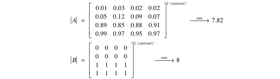
For the case of evaluating a Dice coefficient on predicted segmentation masks, we can approximate $\left|A\cap B\right|$ as the element-wise multiplication between the prediction and target mask, and then sum the resulting matrix.

Because our target mask is binary, we effectively zero-out any pixels from our prediction which are not "activated" in the target mask. For the remaining pixels, we are essentially penalizing low-confidence predictions; a higher value for this expression, which is in the numerator, leads to a better Dice coefficient.

In order to quantify $\left|A\right|$ and $\left|B\right|$, some researchers use the simple sum whereas other researchers prefer to use the squared sum for this calculation. I don't have the practical experience to know which performs better empirically over a wide range of tasks, so I'll leave you to try them both and see which works better.

In case you were wondering, there's a 2 in the numerator in calculating the Dice coefficient because our denominator "double counts" the common elements between the two sets. In order to formulate a loss function which can be minimized, we'll simply use $1-Dice$. This loss function is known as the soft Dice loss because we directly use the predicted probabilities instead of thresholding and converting them into a binary mask.

With respect to the neural network output, the numerator is concerned with the common activations between our prediction and target mask, where as the denominator is concerned with the quantity of activations in each mask separately. This has the effect of normalizing our loss according to the size of the target mask such that the soft Dice loss does not struggle learning from classes with lesser spatial representation in an image.

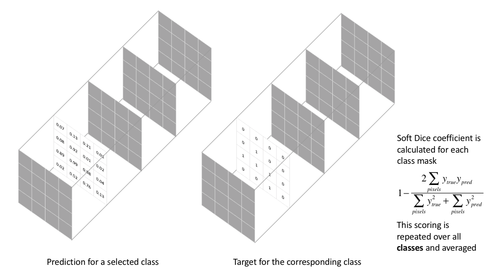
A soft Dice loss is calculated for each class separately and then averaged to yield a final score. An example implementation is provided below.

Common datasets and segmentation competitions

Below, I've listed a number of common datasets that researchers use to train new models and benchmark against the state of the art. You can also explore previous Kaggle competitions and read about how winning solutions implemented segmentation models for their given task.

Datasets

• PASCAL VOC 2012 Segmentation Competition
• COCO 2018 Stuff Segmentation Task
• BDD100K: A Large-scale Diverse Driving Video Database
• Cambridge-driving Labeled Video Database (CamVid)
• Cityscapes Dataset
• Mapillary Vistas Dataset
• ApolloScape Scene Parsing

Past Kaggle Competitions

• 2018 Data Science Bowl
  • Read about the first place solution.
• Carvana Image Masking Challenge
  • Read about the first place solution.
• Dstl Satellite Imagery Feature Detection
  • Read about the third place solution.

Further Reading

Papers

• Fully Convolutional Networks for Semantic Segmentation
• U-Net: Convolutional Networks for Biomedical Image Segmentation
• The Importance of Skip Connections in Biomedical Image Segmentation
• The One Hundred Layers Tiramisu:
  Fully Convolutional DenseNets for Semantic Segmentation
• Multi-Scale Context Aggregation by Dilated Convolutions
• DeepLab: Semantic Image Segmentation with Deep Convolutional Nets, Atrous Convolution, and Fully Connected CRFs
• Rethinking Atrous Convolution for Semantic Image Segmentation
• Evaluation of Deep Learning Strategies for Nucleus Segmentation in Fluorescence Images

Lectures

• Stanford CS231n: Detection and Segmentation
  • Lecture Slides

Blog posts

• Mat Kelcey's (Twitter Famous) Bee Detector
• Semantic Image Segmentation with DeepLab in TensorFlow
• Going beyond the bounding box with semantic segmentation
• U-Net Case Study: Data Science Bowl 2018
• Lyft Perception Challenge: 4th place solution

Image labeling tools

• labelme: Image Polygonal Annotation with Python

Useful Github repos

• Pytorch implementations