
In previous posts, I've introduced the concept of neural networks and discussed how we can train neural networks.
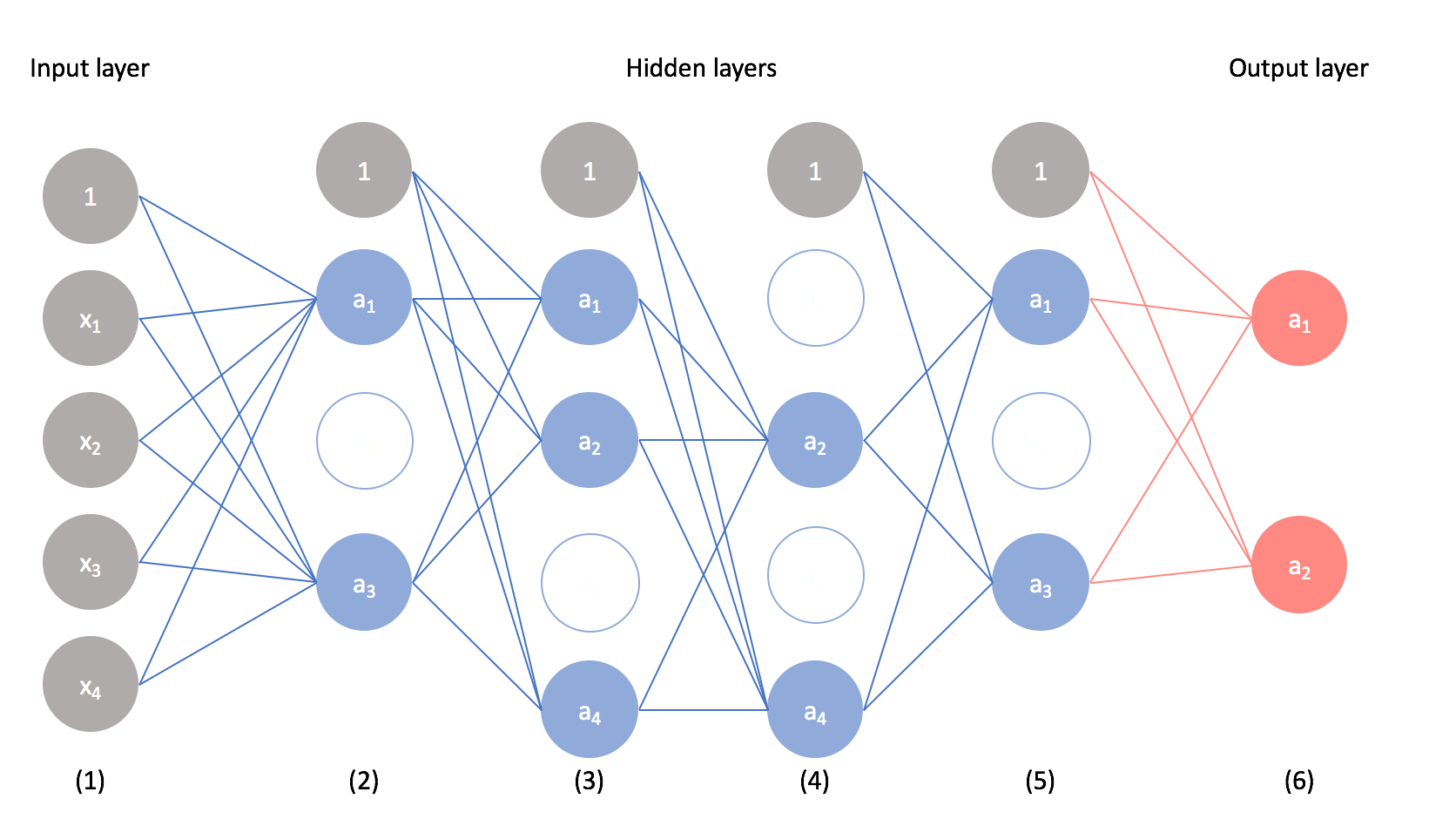
For these posts, we examined neural networks that looked like this.
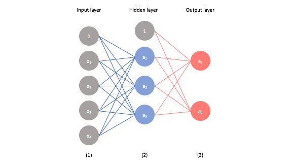
However, many of the modern advancements in neural networks have been a result of stacking many hidden layers.
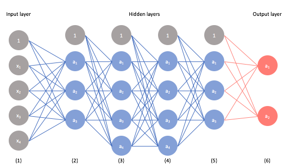
This deep stacking allows us to learn more complex relationships in the data. However, because we're increasing the complexity of the model, we're also more prone to potentially overfitting our data. In this post, I'll discuss common techniques to leverage the power of deep neural networks without falling prey to overfitting.
Early stopping
Arguably, the simplest technique to avoid overfitting is to watch a validation curve while training and stop updating the weights once your validation error starts increasing.
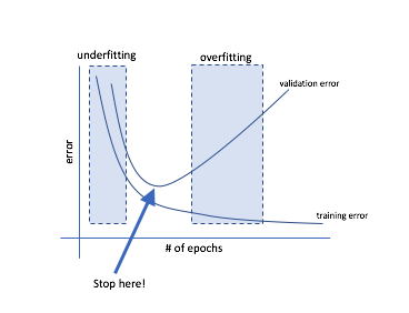
Reminder: During each iteration of training, we perform forward propagation to compute the outputs and backward propagation to compute the errors; one complete iteration over all of the training data is known as an epoch. It is common to report evaluation metrics after each epoch so that we can watch the evolution of our neural network as it trains.
Parameter Regularization
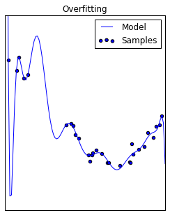
Think back to the overfitting example for linear regression, and recall that this model performs poorly because it suffers from high variance. That is, for small changes in the input value, we see wild fluctuations in the corresponding output. This same problem can occur in neural networks where inputs are linearly combined with parameters to pass information between layers; when these parameters are excessively large, they amplify small changes in the input.
One way to combat this is by penalize parameters in our cost function to prevent parameters from becoming excessively large during training. We can do this via a number of expressions, the two most common are L1 and L2 norms.
L1 regularization
[\lambda \sum\limits_{i = 1}^n {\left| {{\theta_i}} \right|} ]
This expression is commonly used for feature selection as it tends to produce sparse parameter vectors where only the important features take on non-zero values.
L2 regularization
[\lambda \sum\limits_{i = 1}^n {\theta_i^2} ]
This expression doesn't tend to push less important weights to zero and typically produces better results when training a model.
For example, if we select binary cross-entropy with L1 regularization as our loss function, the total expression would be
[J\left( \theta \right) = - \frac{1}{m}\sum\limits _{i = 1}^m {\left[ {{y _i}\ln {{\hat y} _i} + \left( {1 - {y _i}} \right)\ln \left( {1 - {{\hat y} _i}} \right)} \right]} + \lambda \sum\limits _{i = 1}^n {\left| {{\theta _i}} \right|} ]
where the first term in the cost function represents the binary cross-entropy and the second term is our regularization expression. $\lambda$ controls the degree to which we choose to penalize large parameters.
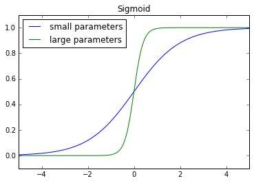
Why do we need to worry about parameters growing excessively large? A neuron's output (activation) is a function of activating a linear combination of inputs and weights to that neuron.
[a = g\left( {{\theta _0} + {\theta _1}{x _1} + {\theta _2}{x _2} + ... + {\theta _n}{x _n}} \right)]
Suppose the case where we have an output neuron which performs binary classification of whether or not an image contains a cat. The output neuron should produce a value close to 1 for cases where image contains a cat and produce values close to 0 for cases where the image does not contain a cat. We measure the performance of this neural network by comparing the output of the neuron to the true label. The true label will always be either 0 or 1, thus our model is incentivized to produce outputs as close to 0 or as close to 1 as possible. One way to accomplish this is by simply increasing the magnitude of the weights. As you can see below, large parameter values have the effect of pushing input closer to 0 and 1; in effect, this arbitrarily increases the confidence in our predictions.
In summary, our model might let parameters grow excessively large to reduce training error but we'd like to prevent this to reduce the variance of our model. We accomplish this by adding a penalty term for large parameter values in our cost function.
Dropout
Ensemble learning is a very intuitive approach to addressing the problem of overfitting. If the problem of overfitting is due to our model learning too much from the training data, we can fix that by training multiple models, each of which learn from the data in different ways. If each component model learns a relationship from the data that contains the true signal with some addition of noise, a combination of models should maintain the relationship of the signal within the data while averaging out the noise.
However, training neural networks is computationally expensive - some neural networks take days to train! Training an ensemble of neural networks? Yeah, that sounds like a terrible idea.
But the concept of ensemble learning to address the overfitting problem still sounds like a good idea... this is where the idea of dropout saves the day for neural networks.
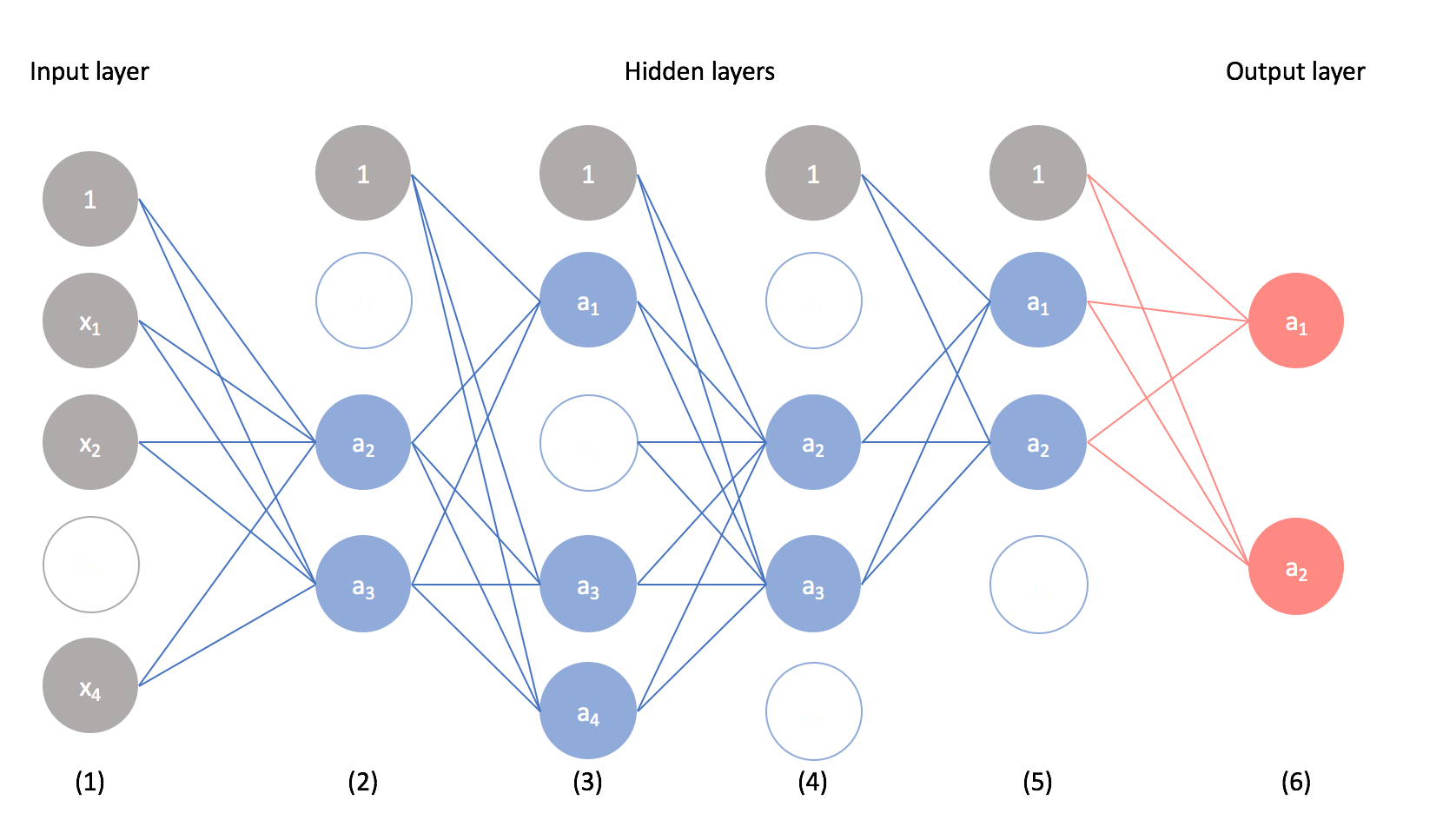
Using dropout, we can build multiple representations of the relationship present in the data by randomly dropping neurons from the network during training. We use a Bernoulli distribution to decide which neurons should be dropped, defining the probability that any given neuron will be dropped as a parameter.
The result is a "thinned" network.
Note: In order to prevent scale problems at test time, the activations of the remaining neurons are upscaled by the dropout factor.
Recomputing dropout during training allows us to build multiple, unique models to learn from the data. You can perform dropout on any layer, visible or hidden.
Unlike other ensemble learners (ex. random forests) where you must keep the collection of models for later use, once you have completed training you can combine the learned parameters from the component models to build a single network with all neurons present.
If you ever need a definition of dropout that is both concise and accurate: pic.twitter.com/D3M7cWbfXY
— Smerity (@Smerity) March 31, 2018
Dropout has brought significant advances to modern neural networks and it considered one of the most powerful techniques to avoid overfitting.