Soft clustering with Gaussian mixed models (EM).

Sometimes when we're performing clustering on a dataset, there exist points which don't belong strongly to any given cluster. If we were to use something like k-means clustering, we're forced to make a decision as to which group an observation belongs to. However, it would be useful to be able to quantify the likelihood of a given observation belonging to any of the clusters present in our dataset. We would then be able to see some observations are a close tie between belonging to two clusters.
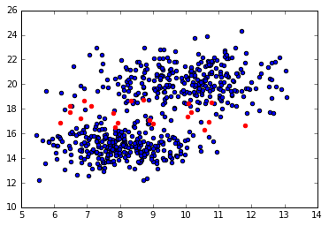
For example, examine the scatterplot showing two clusters (in blue) and some fringe observations (in red) that may belong to either of the two clusters. Ideally, we'd like to be as true to the data as possible when assigning observations to clusters; allowing partial assignment to multiple clusters allows us to more accurately describe the data.
This is accomplished by soft clustering of the data. Formally, soft clustering (also known as fuzzy clustering) is a form clustering where observations may belong to multiple clusters. Today, I'll be writing about a soft clustering technique known as expectation maximization (EM) of a Gaussian mixture model.
Essentially, the process goes as follows:
- Identify the number of clusters you'd like to split the dataset into.
- Define each cluster by generating a Gaussian model.
- For every observation, calculate the probability that it belongs to each cluster (ex. Observation 23 has a 21% chance that it belongs to Cluster A, a 0.1% chance that it belongs to Cluster B, a 48% chance of Cluster C, ... and so forth).
- Using the above probabilities, recalculate the Gaussian models.
- Repeat until observations more or less "converge" on their assignments.
Let's look at a very simple example.
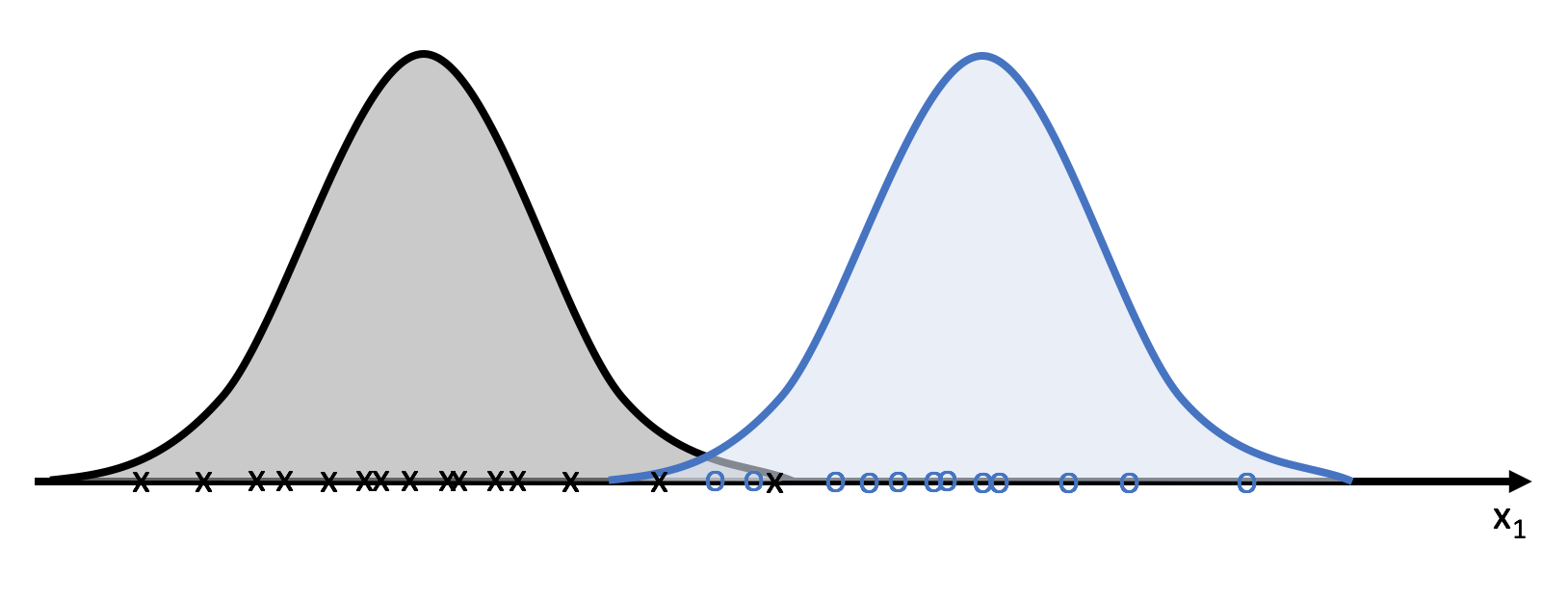
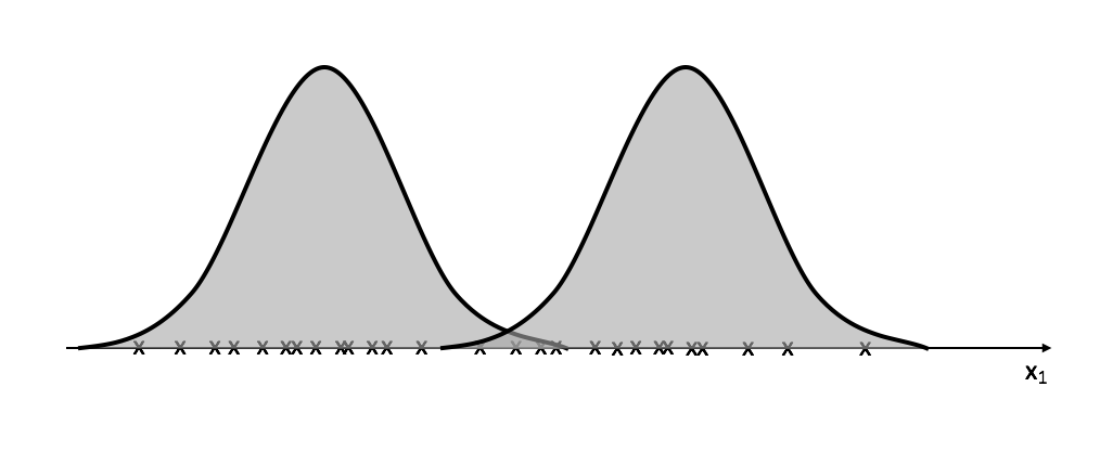
Suppose I have data for a set of observations with one feature, $x _1$, that come from two distinct classes.

We can use this data to build a Gaussian model for each class which would allow us to calculate the probability of a new observation belonging to each class. The class denoted by black x's would be used to build one Gaussian model and the class denoted by blue o's would be used to build a separate Gaussian model. A Gaussian model may be defined by calculating the mean and variance of a dataset; we'll do this twice, once for each class.
For those needing a refresher in statistics, we'll use the probability distribution function to quantify the probability of an observation belongs to a certain cluster.
Unfortunately, we usually perform clustering because we don't have a labeled dataset and thus don't know which class any of the observations belong to- that's what we're hoping to learn!

Since we don't know which class each observation belongs to, we don't have an easy way to build multiple Gaussian models to partition the data. We can no longer simply calculate the mean and variance of observations belonging to each class.
Let's start with a random guess of our Gaussian models and then iteratively optimize the attributes, in a similar fashion as we did for k-mean clustering, to find the optimal Gaussian model to express the data.
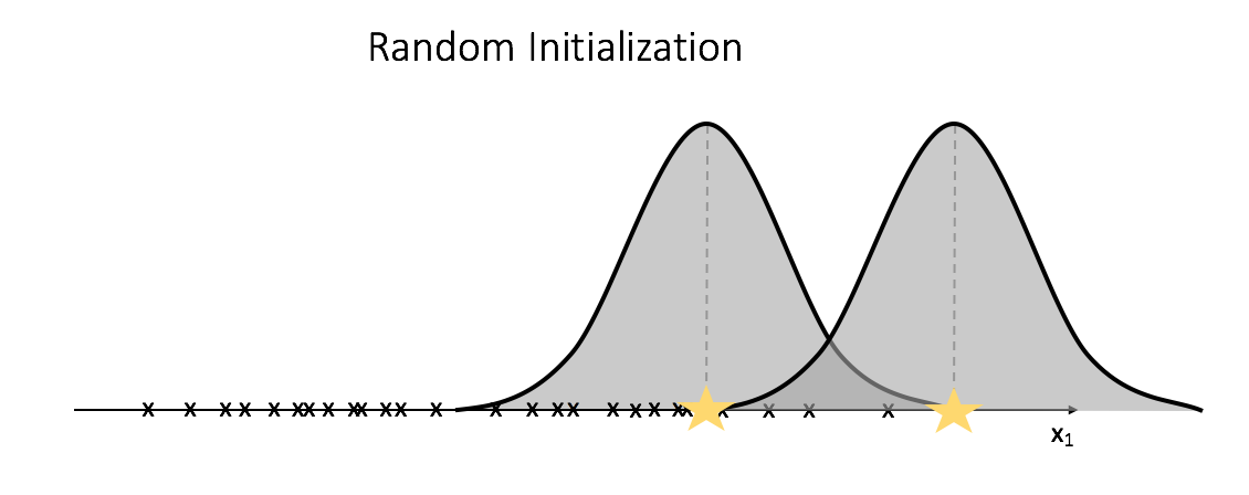
After initializing two random Gaussians, we'll compute the likelihood of each observation being expressed in both of the Gaussian models. We'll then recalculate the Gaussian models; we'll use all of the observations in calculating the mean and variance for each Gaussian, but the observations will be weighted by the likelihood of existing in the given model.
As I mentioned earlier, rather than assigning observations to a class, we'll assume there's a possibility that it can belong to any of the $k$ clusters. Thus, for any given observation we'll calculate the probability of it belonging to each of the $k$ clusters. Let's attach a hidden variable to each observation which contains a vector, $z_ i$, to store these probabilities.
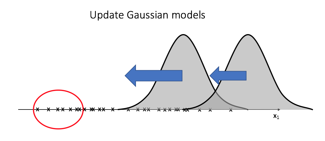
After using $z_i$ to calculate the weighted parameters (mean and variance) for each cluster, we update the Gaussian models. You'll see that the leftmost data (circled below) will pull both models in it's direction, but it will have a larger effect on the left Gaussian since the observations will have a higher weight for the model that it's closest to.
We'll continue this cycle of recalculating $z_i$ and then using it to update the Gaussians until we "converge" on optimal clusters.
The example above visualizes a univariate Gaussian example, we can extend this logic, however, to accomodate multivariate datasets. If you're not familiar with multivariate Gaussian distributions, I recommend you spend a little time reading about them or watching a lecture. I've found this video and this video to be useful. There are subtle difference between univariate and multivariate models, namely that we now have a vector of means and a covariance matrix rather than single values for mean and variance.
Now that we understand what's going on, let's dive into the specifics of the algorithm.
Initializing the clusters
Foremost, we must select how many segments we'd like to partition our data into. To do this, we can use the Bayesian information criterion (BIC). This criterion is commonly used for model selection with preference for the model possessing the lowest BIC. The sklearn documentation has a good example on this process.
Note: You can calculate the BIC of a given GaussianMixture in sklearn using the bic() method.
After selecting $k$ segments to partition the data into, we initialize $k$ random Gaussian models.
Probabalistic assignment to clusters (expectation)
After initializing $k$ random Gaussian models we can calculate our expectation of $z _i$, a vector of probabilities that $x _i$ belongs to the $j ^{th}$ cluster for $j=1$ to $j=k.$ As mentioned earlier, we don't know the true probabilitistic cluster assignments for $z$, so we'll start with a guess and iteratively refine it.
$$ E\left[ {z _{i,j}} \right] = \frac{P\left( {x = {x _i}|\mu = {\mu _j}} \right)}{\sum\limits _{m=1}^k {P\left( {x = {x _i}|\mu = {\mu _m}} \right)} } $$
We can calculate the probability of $x _i$ belonging to cluster $j$ using the probability distribution function of a Gaussian distribution.
[P\left( {x = {x _i}|\mu = {\mu _j}} \right) = \frac{1}{{\sqrt {2\pi {\sigma _j}^2} }}{e^{ - \frac{{^{{{\left( {{x _i} - {\mu _j}} \right)}^2}}}}{{2{\sigma _j}^2}}}}]
Reformulating the Gaussian models (maximization)
We'll then recalculate our Gaussian models leveraging the weights we found in the expectation step. The expectation, ${E\left[ {{z _{i,j}}} \right]}$, represents the likelihood that the $i ^{th}$ observation belongs to cluster $j$.
[{\mu _j} = \frac{{\sum\limits _i {E\left[ {{z _{i,j}}} \right]{x _i}} }}{{\sum\limits _i {E\left[ {{z _{i,j}}} \right]} }}]
[{\sigma _j} = \frac{{\sum\limits _i {E\left[ {{z _{i,j}}} \right]\left( {{x _i} - {\mu _j}} \right)\left( {{x _i} - {\mu _k}} \right)} }}{{\sum\limits _i {E\left[ {{z _{i,j}}} \right]} }}]
Defining a stopping criterion
With k-means clustering, we iteratively recalculated means and reassigned observations until convergence and observations stopped moving between clusters. However, because we're now dealing with continuous probabilities, and because we never give a hard cluster assignment, we can't rely on this convergence. Instead, we'll set a stopping criterion to end the iterative cycle once the observation probabilities stop changing by above some threshold.