Hyperparameter tuning for machine learning models.

When creating a machine learning model, you'll be presented with design choices as to how to define your model architecture. Often times, we don't immediately know what the optimal model architecture should be for a given model, and thus we'd like to be able to explore a range of possibilities. In true machine learning fashion, we'll ideally ask the machine to perform this exploration and select the optimal model architecture automatically. Parameters which define the model architecture are referred to as hyperparameters and thus this process of searching for the ideal model architecture is referred to as hyperparameter tuning.
These hyperparameters might address model design questions such as:
- What degree of polynomial features should I use for my linear model?
- What should be the maximum depth allowed for my decision tree?
- What should be the minimum number of samples required at a leaf node in my decision tree?
- How many trees should I include in my random forest?
- How many neurons should I have in my neural network layer?
- How many layers should I have in my neural network?
- What should I set my learning rate to for gradient descent?
I want to be absolutely clear, hyperparameters are not model parameters and they cannot be directly trained from the data. Model parameters are learned during training when we optimize a loss function using something like gradient descent.The process for learning parameter values is shown generally below.
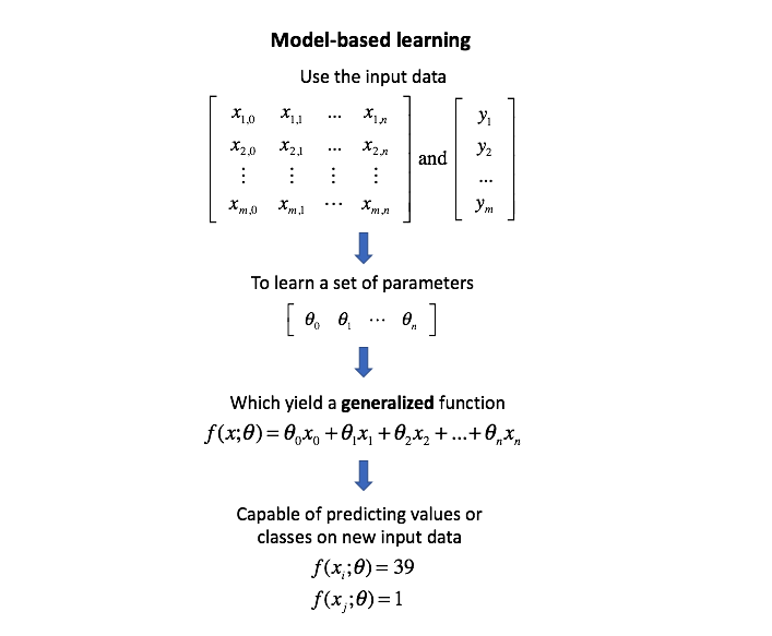
Whereas the model parameters specify how to transform the input data into the desired output, the hyperparameters define how our model is actually structured. Unfortunately, there's no way to calculate “which way should I update my hyperparameter to reduce the loss?” (ie. gradients) in order to find the optimal model architecture; thus, we generally resort to experimentation to figure out what works best.
In general, this process includes:
- Define a model
- Define the range of possible values for all hyperparameters
- Define a method for sampling hyperparameter values
- Define an evaluative criteria to judge the model
- Define a cross-validation method
Specifically, the various hyperparameter tuning methods I'll discuss in this post offer various approaches to Step 3.
Model validation
Before we discuss these various tuning methods, I'd like to quickly revisit the purpose of splitting our data into training, validation, and test data. The ultimate goal for any machine learning model is to learn from examples in such a manner that the model is capable of generalizing the learning to new instances which it has not yet seen. At a very basic level, you should train on a subset of your total dataset, holding out the remaining data for evaluation to gauge the model's ability to generalize - in other words, "how well will my model do on data which it hasn't directly learned from during training?"
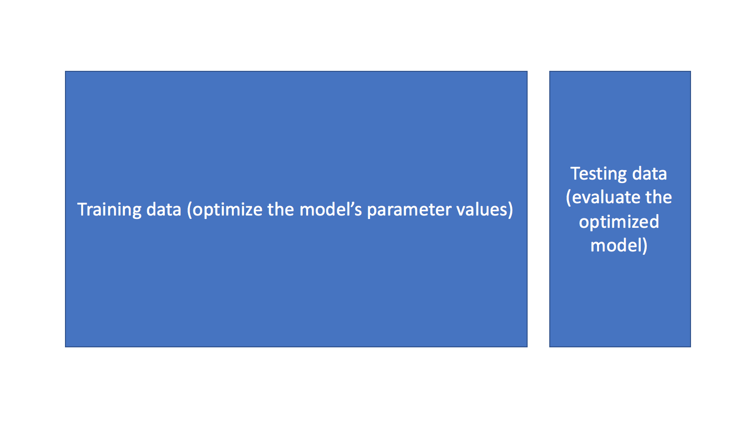
When you start exploring various model architectures (ie. different hyperparameter values), you also need a way to evaluate each model's ability to generalize to unseen data. However, if you use the testing data for this evaluation, you'll end up "fitting" the model architecture to the testing data - losing the ability to truely evaluate how the model performs on unseen data. This is sometimes referred to as "data leakage".
To mitigate this, we'll end up splitting the total dataset into three subsets: training data, validation data, and testing data. The introduction of a validation dataset allows us to evaluate the model on different data than it was trained on and select the best model architecture, while still holding out a subset of the data for the final evaluation at the end of our model development.
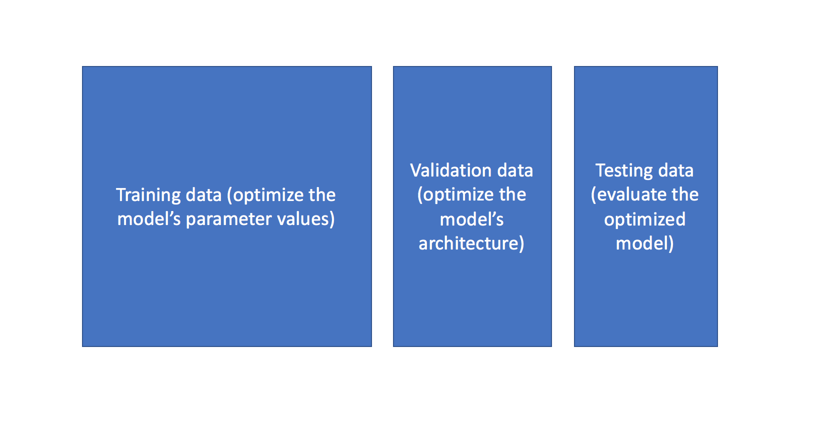
You can also leverage more advanced techniques such as K-fold cross validation in order to essentially combine training and validation data for both learning the model parameters and evaluating the model without introducing data leakage.
Hyperparameter tuning methods
Recall that I previously mentioned that the hyperparameter tuning methods relate to how we sample possible model architecture candidates from the space of possible hyperparameter values. This is often referred to as "searching" the hyperparameter space for the optimum values. In the following visualization, the $x$ and $y$ dimensions represent two hyperparameters, and the $z$ dimension represents the model's score (defined by some evaluation metric) for the architecture defined by $x$ and $y$.
Note: Ignore the axes values, I borrowed this image as noted and the axis values don't correspond with logical values for the hyperparameters.
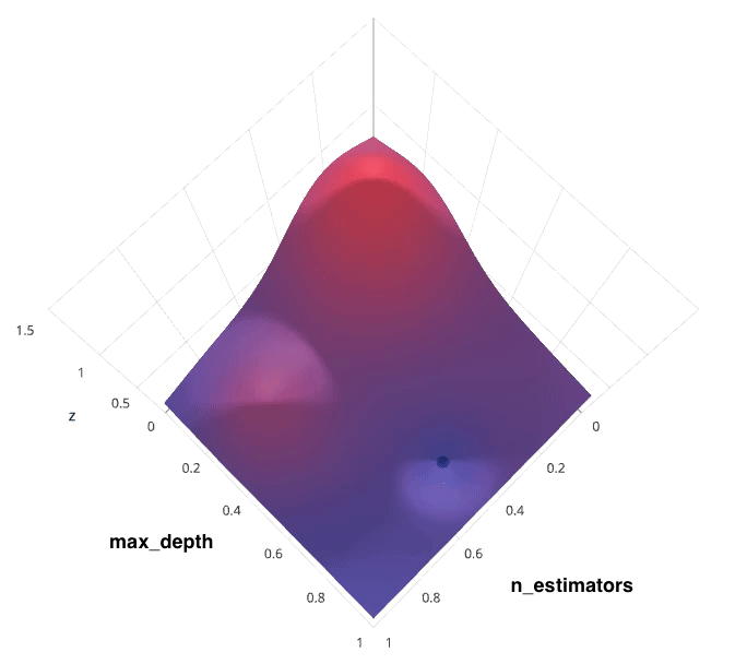
Photo by SigOpt
If we had access to such a plot, choosing the ideal hyperparameter combination would be trivial. However, calculating such a plot at the granularity visualized above would be prohibitively expensive. Thus, we are left to blindly explore the hyperparameter space in hopes of locating the hyperparameter values which lead to the maximum score.
For each method, I'll discuss how to search for the optimal structure of a random forest classifer. Random forests are an ensemble model comprised of a collection of decision trees; when building such a model, two important hyperparameters to consider are:
- How many estimators (ie. decision trees) should I use?
- What should be the maximum allowable depth for each decision tree?
Grid search
Grid search is arguably the most basic hyperparameter tuning method. With this technique, we simply build a model for each possible combination of all of the hyperparameter values provided, evaluating each model, and selecting the architecture which produces the best results.
For example, we would define a list of values to try for both n_estimators and max_depth and a grid search would build a model for each possible combination.
Performing grid search over the defined hyperparameter space
n_estimators = [10, 50, 100, 200]
max_depth = [3, 10, 20, 40]
would yield the following models.
RandomForestClassifier(n_estimators=10, max_depth=3)
RandomForestClassifier(n_estimators=10, max_depth=10)
RandomForestClassifier(n_estimators=10, max_depth=20)
RandomForestClassifier(n_estimators=10, max_depth=40)

RandomForestClassifier(n_estimators=50, max_depth=3)
RandomForestClassifier(n_estimators=50, max_depth=10)
RandomForestClassifier(n_estimators=50, max_depth=20)
RandomForestClassifier(n_estimators=50, max_depth=40)

RandomForestClassifier(n_estimators=100, max_depth=3)
RandomForestClassifier(n_estimators=100, max_depth=10)
RandomForestClassifier(n_estimators=100, max_depth=20)
RandomForestClassifier(n_estimators=100, max_depth=40)

RandomForestClassifier(n_estimators=200, max_depth=3)
RandomForestClassifier(n_estimators=200, max_depth=10)
RandomForestClassifier(n_estimators=200, max_depth=20)
RandomForestClassifier(n_estimators=200, max_depth=40)
Each model would be fit to the training data and evaluated on the validation data. As you can see, this is an exhaustive sampling of the hyperparameter space and can be quite inefficient.
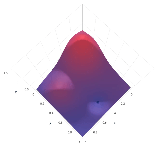
Photo by SigOpt
Random search
Random search differs from grid search in that we longer provide a discrete set of values to explore for each hyperparameter; rather, we provide a statistical distribution for each hyperparameter from which values may be randomly sampled.
We'll define a sampling distribution for each hyperparameter.
from scipy.stats import expon as sp_expon
from scipy.stats import randint as sp_randint

n_estimators = sp_expon(scale=100)
max_depth = sp_randint(1, 40)
We can also define how many iterations we'd like to build when searching for the optimal model. For each iteration, the hyperparameter values of the model will be set by sampling the defined distributions above. The scipy distributions above may be sampled with the rvs() function - feel free to explore this in Python!
One of the main theoretical backings to motivate the use of random search in place of grid search is the fact that for most cases, hyperparameters are not equally important.
A Gaussian process analysis of the function from hyper-parameters to validation set performance reveals that for most data sets only a few of the hyper-parameters really matter, but that different hyper-parameters are important on different data sets. This phenomenon makes grid search a poor choice for configuring algorithms for new data sets. - Bergstra, 2012
In the following example, we're searching over a hyperparameter space where the one hyperparameter has significantly more influence on optimizing the model score - the distributions shown on each axis represent the model's score. In each case, we're evaluating nine different models. The grid search strategy blatantly misses the optimal model and spends redundant time exploring the unimportant parameter. During this grid search, we isolated each hyperparameter and searched for the best possible value while holding all other hyperparameters constant. For cases where the hyperparameter being studied has little effect on the resulting model score, this results in wasted effort. Conversely, the random search has much improved exploratory power and can focus on finding the optimal value for the important hyperparameter.
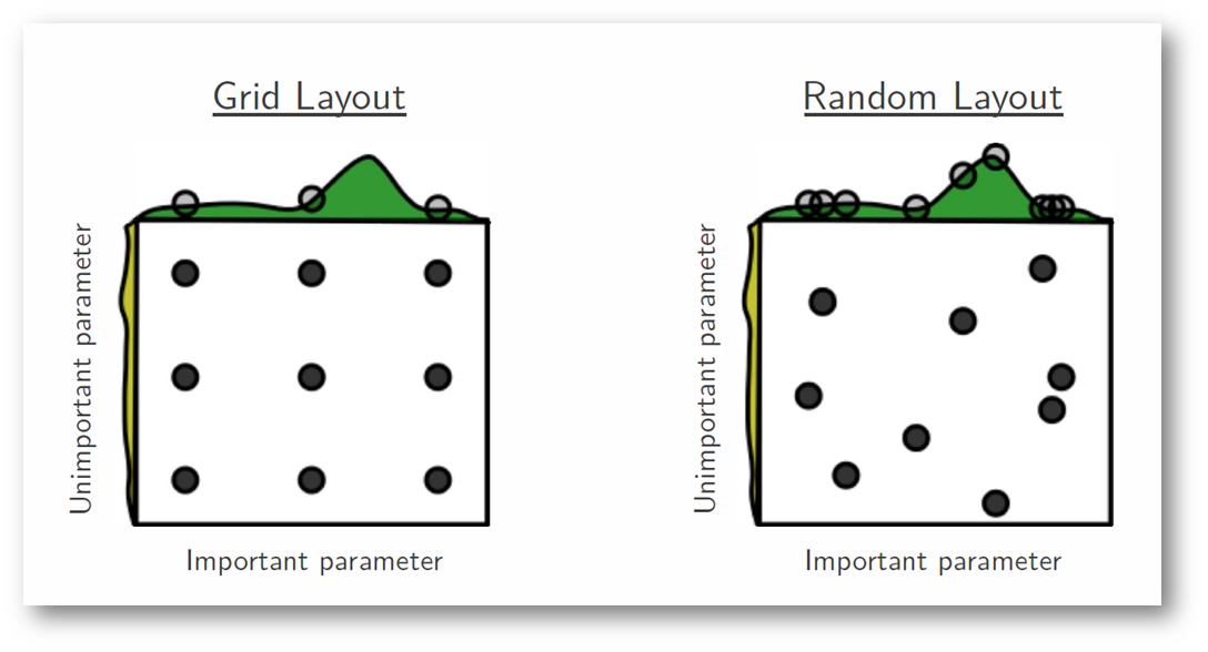
Photo by Bergstra, 2012
As you can see, this search method works best under the assumption that not all hyperparameters are equally important. While this isn't always the case, the assumption holds true for most datasets.
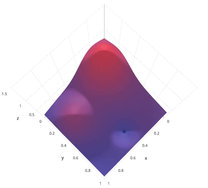
Photo by SigOpt
Bayesian optimization
The previous two methods performed individual experiments building models with various hyperparameter values and recording the model performance for each. Because each experiment was performed in isolation, it's very easy to parallelize this process. However, because each experiment was performed in isolation, we're not able to use the information from one experiment to improve the next experiment. Bayesian optimization belongs to a class of sequential model-based optimization (SMBO) algorithms that allow for one to use the results of our previous iteration to improve our sampling method of the next experiment.
We'll initially define a model constructed with hyperparameters $\lambda$ which, after training, is scored $v$ according to some evaluation metric. Next, we use the previously evaluated hyperparameter values to compute a posterior expectation of the hyperparameter space. We can then choose the optimal hyperparameter values according to this posterior expectation as our next model candidate. We iteratively repeat this process until converging to an optimum.
We'll use a Gaussian process to model our prior probability of model scores across the hyperparameter space. This model will essentially serve to use the hyperparameter values $\lambda_{1,...i}$ and corresponding scores $v_{1,...i}$ we've observed thus far to approximate a continuous score function over the hyperparameter space. This approximated function also includes the degree of certainty of our estimate, which we can use to identify the candidate hyperparameter values that would yield the largest expected improvement over the current score. The formulation for expected improvemenet is known as our acquisition function, which represents the posterior distribution of our score function across the hyperparameter space.

Photo by SigOpt
Note: these visualizations were provided by SigOpt, a company that offers a Bayesian optimization product. It's not likely a coincidence that the visualized hyperparamter space is such that Bayesian optimization performs best.
Further reading
- Random Search for Hyper-Parameter Optimization
- Tuning the hyper-parameters of an estimator
- A Conceptual Explanation of Bayesian Hyperparameter Optimization for Machine Learning
- Common Problems in Hyperparameter Optimization
- Gilles Louppe | Bayesian optimization with Scikit-Optimize
- Hyperparameter Optimization with Keras
- A Tutorial on Bayesian Optimization of Expensive Cost Functions, with Application to Active User Modeling and Hierarchical Reinforcement Learning
- Population based training of neural networks
Hyperparameter optimization libraries (free and open source):
- Ray.tune: Hyperparameter Optimization Framework
- Optuna
- Hyperopt
- Polyaxon
- Talos
- BayesianOptimization
- Metric Optimization Engine
- Spearmint
- GPyOpt
- Scikit-Optimize
Hyperparameter optimization libraries (everybody's favorite commerial library):
Implementation examples: