Logistic regression.

The goal of logistic regression, as with any classifier, is to figure out some way to split the data to allow for an accurate prediction of a given observation's class using the information present in the features. (For instance, if we were examining the Iris flower dataset, our classifier would figure out some method to split the data based on the following: sepal length, sepal width, petal length, petal width.) In the case of a generic two-dimensional example, the split might look something like this.
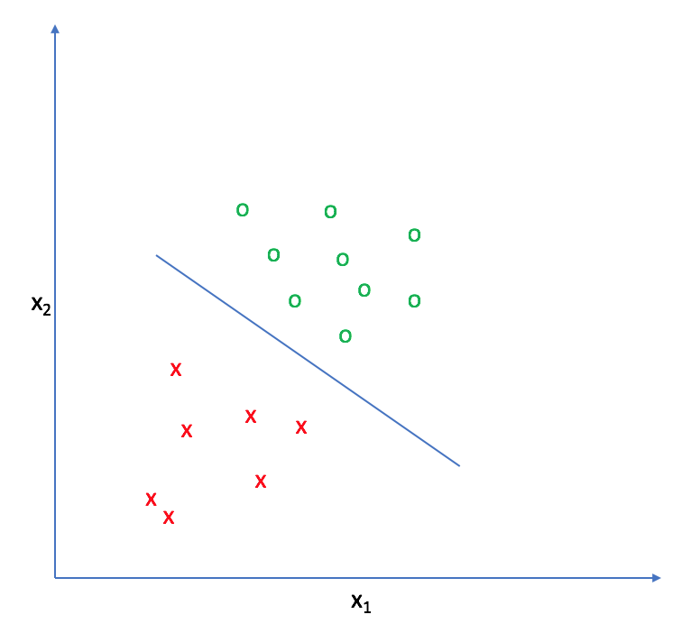
The decision boundary
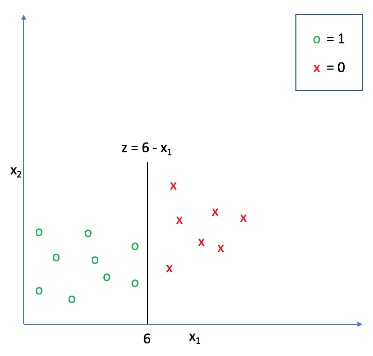
Let's suppose we define a line that is equal to zero along this decision boundary. This way, all of the points on one side of the line take on positive values and all of the points on the other side take on negative values.
For example, in the following graph, $z = 6 - {x _1}$ represents a decision boundary for which any values of ${x _1} > 6$ will return a negative value for $z$ and any values of ${x _1} < 6$ will return a positive value for $z$.
We can extend this decision boundary representation as any linear model, with or without additional polynomial features. (If this model representation doesn't look familiar, check out my post on linear regression).
$$z\left( x \right) = {\theta _0} + {\theta _1}{x _1} + {\theta _2}{x _2} + ... + {\theta _n}{x _n} = {\theta ^T}x$$
Adding polynomial features allows us to construct nonlinear splits in the data in order to draw a more accurate decision boundary.
As we continue, think of $z\left( x \right)$ as a measure of how far a certain data point exists from the decision boundary.
The logistic function
Next, let's take a look at the logistic function.
$$g\left( z \right) = \frac{1}{{1 + {e^{ - z}}}}$$
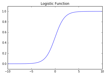
As you can see, this function is asymptotically bounded between 0 and 1. Further, for very positive inputs our output will be close to 1 and for very negative inputs our output will be close to 0. This will essentially allow us to translate the value we obtain from $z$ into a prediction of the proper class. Inputs that are close to zero (and thus, near the decision boundary) signify that we don't have a confident prediction of 0 or 1 for the observation.
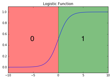
At the decision boundary $z=0$, the function $g\left( z \right) = 0.5$. We'll use this value as a cutoff establishing the prediction criterion:
$${h _\theta }({x _i}) \ge 0.5 \to {y _{pred}} = 1$$
$${h _\theta }({x _i}) < 0.5 \to {y _{pred}} = 0$$
where ${y _{pred}}$ denotes the predicted class of an observation, ${x _i}$, and ${h _\theta }({x})$ represents the functional composition, ${h _\theta }\left( x \right) = g\left( {z\left( x \right)} \right)$.
More concretely, we can write our model as:
$${h_\theta }\left( x \right) = \frac{1}{{1 + {e^{ - {\theta ^T}x}}}}$$
Thus, the output of this function represents a binary prediction for the input observation's class.
Another way to interpret this output is to view it in terms of a probabilistic prediction of the true class. In other words, ${h _\theta }\left( x \right)$ represents the estimated probability that ${y _i} = 1$ for a given input, ${x _i}$.
$${h _\theta }\left( {{x _i}} \right) = {\rm{P}}\left( {{y _i} = 1|{x _i};\theta } \right)$$
Because the class can only take on values of 0 or 1, we can also write this in terms of the probability that ${y _i} = 0$ for a given input, ${x _i}$.
$${\rm{P}}\left( {{y _i} = 0|{x _i};\theta } \right) = 1 - {\rm{P}}\left( {{y _i} = 1|{x _i};\theta } \right)$$
For example, if ${h _\theta }\left( x \right) = 0.85$ then we can assert that there is an 85% probability that ${y _i} = 1$ and a 15% probability that ${y _i} = 0$. This is useful as we can not only predict the class of an observation, but we can quantify the certainty of such prediction. In essence, the further a point is from the decision boundary, the more certain we are about the decision.
The cost function
Next, we need to establish a cost function which can grade how well our model is performing according to the training data. This cost function, $J\left( \theta \right)$, can be considered to be a summation of individual "grades" for each classification prediction in our training set, comparing ${h_\theta }\left( x \right)$ with the true class $y _i$. We want the cost function to be large for incorrect classifications and small for correct ones so that we can minimize $J\left( \theta \right)$ to find the optimal parameters.
$$J\left( \theta \right) = \frac{1}{m}\sum\limits_{i = 1}^m {{\rm{Cost}}({h _\theta }\left( {{x _i}} \right),{y _i})}$$
In linear regression, we used the squared error as our grading mechanism. Unfortunately for logistic regression, such a cost function produces a nonconvex space that is not ideal for optimization. There will exist many local optima on which our optimization algorithm might prematurely converge before finding the true minimum.
Using the Maximum Likelihood Estimator from statistics, we can obtain the following cost function which produces a convex space friendly for optimization. This function is known as the binary cross-entropy loss.
These cost functions return high costs for incorrect predictions.
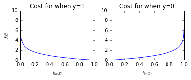
More succinctly, we can write this as
$${\rm{Cost}}({h _\theta }\left( x \right),y) = - y\log \left( {{h _\theta }\left( x \right)} \right) - \left( {1 - y} \right)\log \left( {1 - {h _\theta }\left( x \right)} \right)$$
since the second term will be zero when $y=1$ and the first term will be zero when $y=0$. Substituting this cost into our overall cost function we obtain:
$$J\left( \theta \right) = \frac{1}{m}\sum\limits _{i = 1}^m { - {y _i}\log \left( {{h _\theta }\left( {{x _i}} \right)} \right) - \left( {1 - {y _i}} \right)\log \left( {1 - {h _\theta }\left( {{x _i}} \right)} \right)} $$
Finding the best parameters
Gradient descent
As a reminder, the algorithm for gradient descent is provided below.
$${\theta _j}: = {\theta _j} - \alpha \frac{\partial }{{\partial {\theta _j}}}J\left( \theta \right)$$
Taking the partial derivative of the cost function from the previous section, we find:
$$\frac{\partial }{{\partial {\theta _j}}}J\left( \theta \right) = \frac{1}{m}\sum\limits _{i = 1}^m {\left( {{h _\theta }\left( {{x _i}} \right) - {y _i}} \right)} {x _{i,j}}$$
And thus our parameter update rule for gradient descent is:
$${\theta _j}: = {\theta _j} - \frac{\alpha }{m}\sum\limits _{i = 1}^m {\left( {{h _\theta }\left( {{x _i}} \right) - {y _i}} \right)} {x _{i,j}}$$
Advanced optimizations
In practice, there are more advanced optimization techniques that perform much better than gradient descent including conjugate gradient, BFGS, and L-BFGS. These advanced numerical techniques are not within the current scope of this blog post.
In sklearn's implementation of logistic regression, you can define which optimization is used with the solver parameter.
Multiclass classification
While binary classification is useful, it'd be really nice to be able to train a classifier that can separate the data into more than two classes. For example, the Iris dataset I mentioned in the beginning of this post has three target classes: Iris Setosa, Iris Versicolour, and Iris Virginica. A simple binary classifier simply wouldn't work for this dataset!
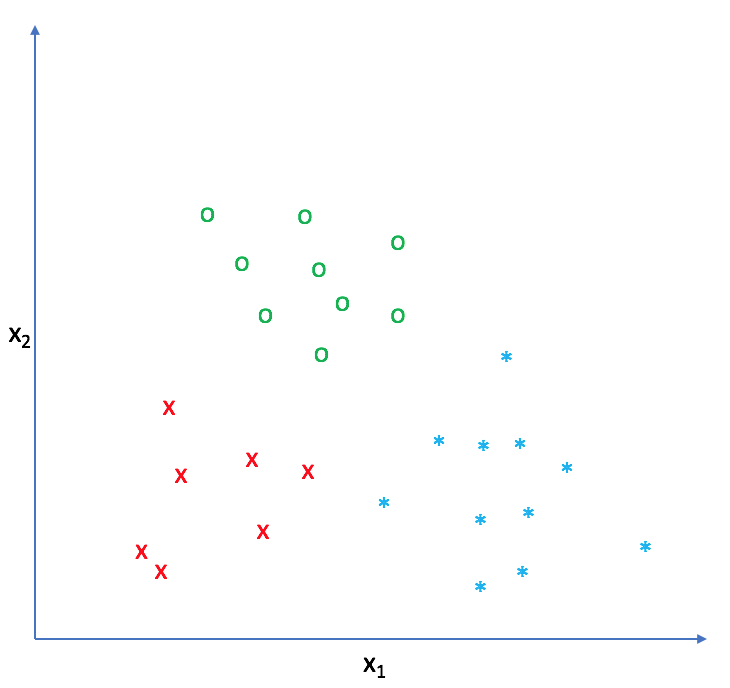
However, using a one-vs-all (also known as one-vs-rest) classifier we can use a combination of binary classifiers for multiclass classification. We simply look at each class, one by one, and treat all of the other classes as the same. In a sense, you look at "Class 1" and build a classifier that can predict "Class 1" or "Not Class 1", and then do the same for each class that exists in your dataset.
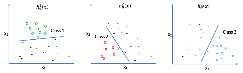
In other words, each classifier $h _\theta ^i\left( x \right)$ returns the probability that an observation belongs to class $i$. Therefore, all we have to do in order to predict the class of an observation is to select the class of whichever classifier returns the highest probability.
Summary
Each example has an $n$ dimensional feature vector, ${x _i}$, which belongs to a class, ${y _i}$.
Our hypothesis function predicts the likelihood that the example $i$ belongs to the class ${y _i}=1$
$${h _\theta }\left( x \right) = \frac{1}{{1 + {e^{ - {\theta ^T}x}}}}$$
where $\theta ^Tx$ represents a decision boundary. We can assign a cost function to optimize the parameters $\theta$ to provide the best possible decision boundary.
In order to build a classifier capable of distinguishing between more than two classes, we simply build a collection of classifiers which each return the probability the observation belongs to a specific class.
For a dataset with $k$ classes, you'd train a collection of $k$ classifiers.
$$h _\theta ^1\left( x \right),h _\theta ^2\left( x \right),...h _\theta ^k\left( x \right)$$